9. Stochastic Methods: Exercise

Name:

import numpy as np
import matplotlib.pyplot as plt
%matplotlib inline

1. Integration

When an explicit function like \(x_n = g(x_1,...,x_{n-1})\) is not available, you can use a binary function that takes 1 within and 0 outside of a region to measure its volume.

1. Measure the volume of an n-dimensional sphere using a binary function

\[\begin{split} f(x) = \left\{ \begin{array}{ccc} 1 & \mbox{if} & \sum_{i=1}^n x_i^2 \le 1 \\ 0 & \mbox{otherwise} & \end{array}\right. \end{split}\]

2. Measure the area or volume of a shape of your interest by sampling method.

2. Rejection Sampling

Let us generate samples from Gamma distribution

\[ p(x; k, \theta) = \frac{1}{\Gamma(k)\theta^k}x^{k-1}e^{-\frac{x}{\theta}} \]

with the shape parameter \(k>0\) and the scaling parameter \(\theta\) using the gamma function \(\Gamma(k)\) available in scipy.special.

from scipy.special import gamma
from scipy.special import factorial

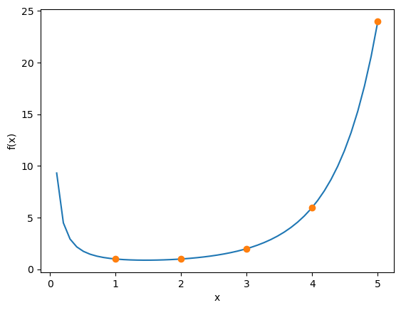
Here is how the gamma function looks like, together with factorial at integer values.

kmax = 5
x = np.linspace(0, kmax, 50)
plt.plot(x, gamma(x))
plt.plot(range(1,kmax+1), [factorial(k-1) for k in range(1,kmax+1)], 'o')
plt.xlabel("x"); plt.ylabel("f(x)")

Text(0, 0.5, 'f(x)')

1. Define the Gamma density function with arbitrary \(k\) and \(\theta\).

def p_gamma(x, k=1, theta=1):
    """density function of gamma distribution"""
    
    return 

Consider the exponential distribution \(q(x;\mu)=\frac{1}{\mu}e^{-\frac{x}{\mu}}\) as the proposal distribution.

def p_exp(x, mu=1):
    """density function of exponential distribution"""
    return 

def x_exp(n=1, mu=1):
    """sample from exponential distribution"""
    y = np.random.random(n)  # uniform in [0,1]
    return 

The ratio of the target and proposal distributions is

\[ \frac{p(x;k,\theta)}{q(x;\mu)} = \frac{\mu}{\Gamma(k)\theta^k}x^{k-1}e^{(\frac{1}{\mu}-\frac{1}{\theta})x}. \]

By setting

\[ \frac{d}{dx}\frac{p(x;k,\theta)}{q(x;\mu)} = 0 \]

we have

\[ \{(k-1)x^{k-2}+(\frac{1}{\mu}-\frac{1}{\theta})x^{k-1}\}e^{(\frac{1}{\mu}-\frac{1}{\theta})x} = 0. \]

Thus at

\[ x = \frac{(k-1)\mu\theta}{\mu-\theta} \]

the ratio \(\frac{p(x;k,\theta)}{q(x;\mu)}\) takes the maximum

\[ \frac{\mu^k}{\Gamma(k)\theta}\left(\frac{k-1}{\mu-\theta}\right)^{k-1}e^{1-k}. \]

2. What is a good choice of \(\mu\) to satisfy \(p(x)\le cq(x)\) and what is the value of \(c\) for that?

By setting \(\mu=k\theta\), we have \(p(x)\le cq(x)\) with \(c=\frac{k^k}{\Gamma(k)}e^{1-k}\)

3. Verify that \(cq(x)\) covers \(p(x)\) by plotting them for some \(k\) and \(\theta\).

k = 2
theta = 2
c = (k**k)/gamma(k)*np.exp(1-k)
x = np.linspace(0, 10, 50)
plt.plot(x, p_gamma(x, k, theta))
plt.plot(x, c*p_exp(x, k*theta))
plt.xlabel("x");

---------------------------------------------------------------------------
ValueError                                Traceback (most recent call last)
Cell In[6], line 5
      3 c = (k**k)/gamma(k)*np.exp(1-k)
      4 x = np.linspace(0, 10, 50)
----> 5 plt.plot(x, p_gamma(x, k, theta))
      6 plt.plot(x, c*p_exp(x, k*theta))
      7 plt.xlabel("x");

File ~/miniforge3/lib/python3.13/site-packages/matplotlib/pyplot.py:3827, in plot(scalex, scaley, data, *args, **kwargs)
   3819 @_copy_docstring_and_deprecators(Axes.plot)
   3820 def plot(
   3821     *args: float | ArrayLike | str,
   (...)   3825     **kwargs,
   3826 ) -> list[Line2D]:
-> 3827     return gca().plot(
   3828         *args,
   3829         scalex=scalex,
   3830         scaley=scaley,
   3831         **({"data": data} if data is not None else {}),
   3832         **kwargs,
   3833     )

File ~/miniforge3/lib/python3.13/site-packages/matplotlib/axes/_axes.py:1777, in Axes.plot(self, scalex, scaley, data, *args, **kwargs)
   1534 """
   1535 Plot y versus x as lines and/or markers.
   1536 
   (...)   1774 (``'green'``) or hex strings (``'#008000'``).
   1775 """
   1776 kwargs = cbook.normalize_kwargs(kwargs, mlines.Line2D)
-> 1777 lines = [*self._get_lines(self, *args, data=data, **kwargs)]
   1778 for line in lines:
   1779     self.add_line(line)

File ~/miniforge3/lib/python3.13/site-packages/matplotlib/axes/_base.py:297, in _process_plot_var_args.__call__(self, axes, data, return_kwargs, *args, **kwargs)
    295     this += args[0],
    296     args = args[1:]
--> 297 yield from self._plot_args(
    298     axes, this, kwargs, ambiguous_fmt_datakey=ambiguous_fmt_datakey,
    299     return_kwargs=return_kwargs
    300 )

File ~/miniforge3/lib/python3.13/site-packages/matplotlib/axes/_base.py:455, in _process_plot_var_args._plot_args(self, axes, tup, kwargs, return_kwargs, ambiguous_fmt_datakey)
    452 # Don't allow any None value; these would be up-converted to one
    453 # element array of None which causes problems downstream.
    454 if any(v is None for v in tup):
--> 455     raise ValueError("x, y, and format string must not be None")
    457 kw = {}
    458 for prop_name, val in zip(('linestyle', 'marker', 'color'),
    459                           (linestyle, marker, color)):

ValueError: x, y, and format string must not be None

4. Implement a function to general samples from Gamma distribution with arbitorary \(k\) and \(\theta\) using rejection sampling from exponential distribution.

def x_gamma(n=1, k=1, theta=1):
    """sample from gamma distribution by rejection sampling"""
    c = (k**k)/gamma(k)*np.exp(1-k)
    #print("c =", c)
    xe = x_exp(n, k*theta)
    paccept = 
    accept = np.random.random(n)<paccept
    xg = xe[accept]  # rejection sampling
    #print("accept rate =", len(xg)/n)
    return(xg)

k = 2
theta = 2
# sample histogram
xs = x_gamma(1000, k, theta)
plt.hist(xs, bins=20, density=True)
# compare with the density function
x = np.linspace(0, 10, 100)
plt.plot(x, p_gamma(x, k, theta))
plt.xlabel("")

3. Importance Sampling

You have \(m\) sample values \(f(x_i)\) \((i=1,...m)\) at \(x_i\) following a normal distribution

\[ q(x;\mu_0,\sigma_0) = \frac{1}{\sqrt{2\pi \sigma_0^2}}e^{-\frac{(x-\mu_0)^2}{2\sigma_0^2}}. \]

Consider estimating the mean of \(f(x)\) for samples with a different normal distribution \(p(x;\mu_1, \sigma_1)\) by importance sampling

\[ E_p[h(x)] = E_q\left[\frac{p(x)}{q(x)}h(x)\right] \]

1. What is the importance weight \(\frac{p(x)}{q(x)}\)?

2. Let us consider the simplest case of \(f(x)=x\).

Generate \(m=100\) samples with \(\mu_0=100\) and \(\sigma_0=20\) and take the sample mean \(E_q[f(x)]\).

m = 100
mu0 = 100
sig0 = 20
xs = 
# show histogram
plt.hist(xs, bins=20, density=True)
plt.xlabel("x")
# check the sample mean
np.mean(xs)

3. Estimate the mean \(E_p[f(x)]\) for \(\mu_1=120\) and \(\sigma_1=10\) by importance sampling.

mu1 = 120
sig1 = 20
importance = 
mean1 = np.dot(importance, xs)/m
print(mean1)

4. See how the result changes with different settings of \(\mu_1\), \(\sigma_1\) and sample size \(m\).

Optional) Try with a different function \(f(x)\).

4. MCMC

Try applying Metropolis sampling to your own (unnormalized) distribution.