7. Partial Differential Equations: Exercise#
Name:
import numpy as np
import matplotlib.pyplot as plt
%matplotlib inline
from scipy.integrate import odeint
1. Diffusion Equation#
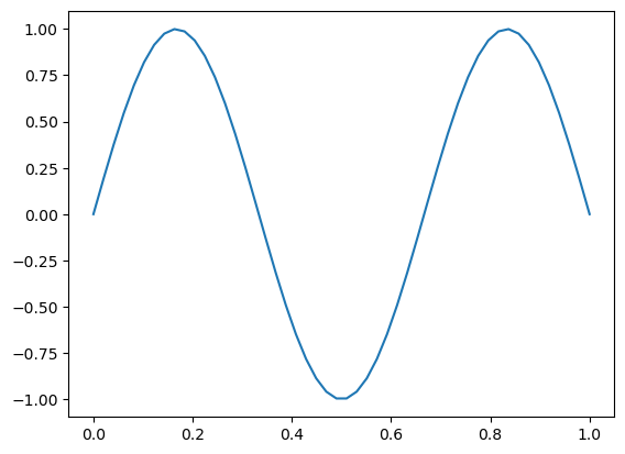
For the diffusion equation with Dirichlet boundary condition, take initial states with different spatial frequencyes, such as
\[ y(x, 0) = \sin(\frac{nx}{L}\pi ) \]
with different \(n\), and see how quickly they decay in time.
L = 1
x = np.linspace(0, L)
n = 3
y = np.sin(n*x*np.pi/L)
plt.plot(x, y)
[<matplotlib.lines.Line2D at 0x124477750>]
2. Wave Equation#
While the wave equation with Dirichlet boundary condition simulates oscillation of a string, that with Neumann condition
\[ \left.\frac{\partial y(x,t)}{\partial x}\right|_{x_0}=\left.\frac{\partial y(x,t)}{\partial x}\right|_{x_N}=0 \]
can simulate water wave.
Implement a wave equation with a decay term
\[ \frac{\partial^2 u}{\partial t^2} = c^2 \frac{\partial^2 u}{\partial x^2} - d \frac{\partial u}{\partial t} \]
with the Neumann boundary conditions and see how the wave ripples.
See how the waves vary with the initial condition or stimulum.
Optional: Wave equation in 2D#
Try simulating waves in a 2D space with a cyclic boundary condition.