2. Visualization: Exercise#
Name:
import numpy as np
import matplotlib.pyplot as plt
%matplotlib inline
1) Plotting curves#
a) Draw a spiral.
b) Draw a “\(\infty\)” shape.
c) Draw a “flower-like” shape.
2) Scatter plots#
Let us take the famous iris data set in scikit-learn package.
from sklearn import datasets
iris = datasets.load_iris()
You can check the description of the data by .DESCR
print(iris.DESCR)
.. _iris_dataset:

Iris plants dataset
--------------------

**Data Set Characteristics:**

:Number of Instances: 150 (50 in each of three classes)
:Number of Attributes: 4 numeric, predictive attributes and the class
:Attribute Information:
    - sepal length in cm
    - sepal width in cm
    - petal length in cm
    - petal width in cm
    - class:
            - Iris-Setosa
            - Iris-Versicolour
            - Iris-Virginica

:Summary Statistics:

============== ==== ==== ======= ===== ====================
                Min  Max   Mean    SD   Class Correlation
============== ==== ==== ======= ===== ====================
sepal length:   4.3  7.9   5.84   0.83    0.7826
sepal width:    2.0  4.4   3.05   0.43   -0.4194
petal length:   1.0  6.9   3.76   1.76    0.9490  (high!)
petal width:    0.1  2.5   1.20   0.76    0.9565  (high!)
============== ==== ==== ======= ===== ====================

:Missing Attribute Values: None
:Class Distribution: 33.3% for each of 3 classes.
:Creator: R.A. Fisher
:Donor: Michael Marshall (MARSHALL%PLU@io.arc.nasa.gov)
:Date: July, 1988

The famous Iris database, first used by Sir R.A. Fisher. The dataset is taken
from Fisher's paper. Note that it's the same as in R, but not as in the UCI
Machine Learning Repository, which has two wrong data points.

This is perhaps the best known database to be found in the
pattern recognition literature.  Fisher's paper is a classic in the field and
is referenced frequently to this day.  (See Duda & Hart, for example.)  The
data set contains 3 classes of 50 instances each, where each class refers to a
type of iris plant.  One class is linearly separable from the other 2; the
latter are NOT linearly separable from each other.

.. dropdown:: References

  - Fisher, R.A. "The use of multiple measurements in taxonomic problems"
    Annual Eugenics, 7, Part II, 179-188 (1936); also in "Contributions to
    Mathematical Statistics" (John Wiley, NY, 1950).
  - Duda, R.O., & Hart, P.E. (1973) Pattern Classification and Scene Analysis.
    (Q327.D83) John Wiley & Sons.  ISBN 0-471-22361-1.  See page 218.
  - Dasarathy, B.V. (1980) "Nosing Around the Neighborhood: A New System
    Structure and Classification Rule for Recognition in Partially Exposed
    Environments".  IEEE Transactions on Pattern Analysis and Machine
    Intelligence, Vol. PAMI-2, No. 1, 67-71.
  - Gates, G.W. (1972) "The Reduced Nearest Neighbor Rule".  IEEE Transactions
    on Information Theory, May 1972, 431-433.
  - See also: 1988 MLC Proceedings, 54-64.  Cheeseman et al"s AUTOCLASS II
    conceptual clustering system finds 3 classes in the data.
  - Many, many more ...
First four columns are:
SepalLength, SepalWidth, PetalLength, PetalWidth
The last column is the flower type:
0:Setosa, 1:Versicolor, 2:Virginica
You can read the actual data by .data and the flower type by .target.
X = iris.data
Y = iris.target
print(X.shape, X, Y)
(150, 4) [[5.1 3.5 1.4 0.2]
 [4.9 3.  1.4 0.2]
 [4.7 3.2 1.3 0.2]
 [4.6 3.1 1.5 0.2]
 [5.  3.6 1.4 0.2]
 [5.4 3.9 1.7 0.4]
 [4.6 3.4 1.4 0.3]
 [5.  3.4 1.5 0.2]
 [4.4 2.9 1.4 0.2]
 [4.9 3.1 1.5 0.1]
 [5.4 3.7 1.5 0.2]
 [4.8 3.4 1.6 0.2]
 [4.8 3.  1.4 0.1]
 [4.3 3.  1.1 0.1]
 [5.8 4.  1.2 0.2]
 [5.7 4.4 1.5 0.4]
 [5.4 3.9 1.3 0.4]
 [5.1 3.5 1.4 0.3]
 [5.7 3.8 1.7 0.3]
 [5.1 3.8 1.5 0.3]
 [5.4 3.4 1.7 0.2]
 [5.1 3.7 1.5 0.4]
 [4.6 3.6 1.  0.2]
 [5.1 3.3 1.7 0.5]
 [4.8 3.4 1.9 0.2]
 [5.  3.  1.6 0.2]
 [5.  3.4 1.6 0.4]
 [5.2 3.5 1.5 0.2]
 [5.2 3.4 1.4 0.2]
 [4.7 3.2 1.6 0.2]
 [4.8 3.1 1.6 0.2]
 [5.4 3.4 1.5 0.4]
 [5.2 4.1 1.5 0.1]
 [5.5 4.2 1.4 0.2]
 [4.9 3.1 1.5 0.2]
 [5.  3.2 1.2 0.2]
 [5.5 3.5 1.3 0.2]
 [4.9 3.6 1.4 0.1]
 [4.4 3.  1.3 0.2]
 [5.1 3.4 1.5 0.2]
 [5.  3.5 1.3 0.3]
 [4.5 2.3 1.3 0.3]
 [4.4 3.2 1.3 0.2]
 [5.  3.5 1.6 0.6]
 [5.1 3.8 1.9 0.4]
 [4.8 3.  1.4 0.3]
 [5.1 3.8 1.6 0.2]
 [4.6 3.2 1.4 0.2]
 [5.3 3.7 1.5 0.2]
 [5.  3.3 1.4 0.2]
 [7.  3.2 4.7 1.4]
 [6.4 3.2 4.5 1.5]
 [6.9 3.1 4.9 1.5]
 [5.5 2.3 4.  1.3]
 [6.5 2.8 4.6 1.5]
 [5.7 2.8 4.5 1.3]
 [6.3 3.3 4.7 1.6]
 [4.9 2.4 3.3 1. ]
 [6.6 2.9 4.6 1.3]
 [5.2 2.7 3.9 1.4]
 [5.  2.  3.5 1. ]
 [5.9 3.  4.2 1.5]
 [6.  2.2 4.  1. ]
 [6.1 2.9 4.7 1.4]
 [5.6 2.9 3.6 1.3]
 [6.7 3.1 4.4 1.4]
 [5.6 3.  4.5 1.5]
 [5.8 2.7 4.1 1. ]
 [6.2 2.2 4.5 1.5]
 [5.6 2.5 3.9 1.1]
 [5.9 3.2 4.8 1.8]
 [6.1 2.8 4.  1.3]
 [6.3 2.5 4.9 1.5]
 [6.1 2.8 4.7 1.2]
 [6.4 2.9 4.3 1.3]
 [6.6 3.  4.4 1.4]
 [6.8 2.8 4.8 1.4]
 [6.7 3.  5.  1.7]
 [6.  2.9 4.5 1.5]
 [5.7 2.6 3.5 1. ]
 [5.5 2.4 3.8 1.1]
 [5.5 2.4 3.7 1. ]
 [5.8 2.7 3.9 1.2]
 [6.  2.7 5.1 1.6]
 [5.4 3.  4.5 1.5]
 [6.  3.4 4.5 1.6]
 [6.7 3.1 4.7 1.5]
 [6.3 2.3 4.4 1.3]
 [5.6 3.  4.1 1.3]
 [5.5 2.5 4.  1.3]
 [5.5 2.6 4.4 1.2]
 [6.1 3.  4.6 1.4]
 [5.8 2.6 4.  1.2]
 [5.  2.3 3.3 1. ]
 [5.6 2.7 4.2 1.3]
 [5.7 3.  4.2 1.2]
 [5.7 2.9 4.2 1.3]
 [6.2 2.9 4.3 1.3]
 [5.1 2.5 3.  1.1]
 [5.7 2.8 4.1 1.3]
 [6.3 3.3 6.  2.5]
 [5.8 2.7 5.1 1.9]
 [7.1 3.  5.9 2.1]
 [6.3 2.9 5.6 1.8]
 [6.5 3.  5.8 2.2]
 [7.6 3.  6.6 2.1]
 [4.9 2.5 4.5 1.7]
 [7.3 2.9 6.3 1.8]
 [6.7 2.5 5.8 1.8]
 [7.2 3.6 6.1 2.5]
 [6.5 3.2 5.1 2. ]
 [6.4 2.7 5.3 1.9]
 [6.8 3.  5.5 2.1]
 [5.7 2.5 5.  2. ]
 [5.8 2.8 5.1 2.4]
 [6.4 3.2 5.3 2.3]
 [6.5 3.  5.5 1.8]
 [7.7 3.8 6.7 2.2]
 [7.7 2.6 6.9 2.3]
 [6.  2.2 5.  1.5]
 [6.9 3.2 5.7 2.3]
 [5.6 2.8 4.9 2. ]
 [7.7 2.8 6.7 2. ]
 [6.3 2.7 4.9 1.8]
 [6.7 3.3 5.7 2.1]
 [7.2 3.2 6.  1.8]
 [6.2 2.8 4.8 1.8]
 [6.1 3.  4.9 1.8]
 [6.4 2.8 5.6 2.1]
 [7.2 3.  5.8 1.6]
 [7.4 2.8 6.1 1.9]
 [7.9 3.8 6.4 2. ]
 [6.4 2.8 5.6 2.2]
 [6.3 2.8 5.1 1.5]
 [6.1 2.6 5.6 1.4]
 [7.7 3.  6.1 2.3]
 [6.3 3.4 5.6 2.4]
 [6.4 3.1 5.5 1.8]
 [6.  3.  4.8 1.8]
 [6.9 3.1 5.4 2.1]
 [6.7 3.1 5.6 2.4]
 [6.9 3.1 5.1 2.3]
 [5.8 2.7 5.1 1.9]
 [6.8 3.2 5.9 2.3]
 [6.7 3.3 5.7 2.5]
 [6.7 3.  5.2 2.3]
 [6.3 2.5 5.  1.9]
 [6.5 3.  5.2 2. ]
 [6.2 3.4 5.4 2.3]
 [5.9 3.  5.1 1.8]] [0 0 0 0 0 0 0 0 0 0 0 0 0 0 0 0 0 0 0 0 0 0 0 0 0 0 0 0 0 0 0 0 0 0 0 0 0
 0 0 0 0 0 0 0 0 0 0 0 0 0 1 1 1 1 1 1 1 1 1 1 1 1 1 1 1 1 1 1 1 1 1 1 1 1
 1 1 1 1 1 1 1 1 1 1 1 1 1 1 1 1 1 1 1 1 1 1 1 1 1 1 2 2 2 2 2 2 2 2 2 2 2
 2 2 2 2 2 2 2 2 2 2 2 2 2 2 2 2 2 2 2 2 2 2 2 2 2 2 2 2 2 2 2 2 2 2 2 2 2
 2 2]
a) Make a scatter plot of the first two columns, with a distinct marker color for each flower type.
b) Create a matrix of pair-wise scatter plots like this:
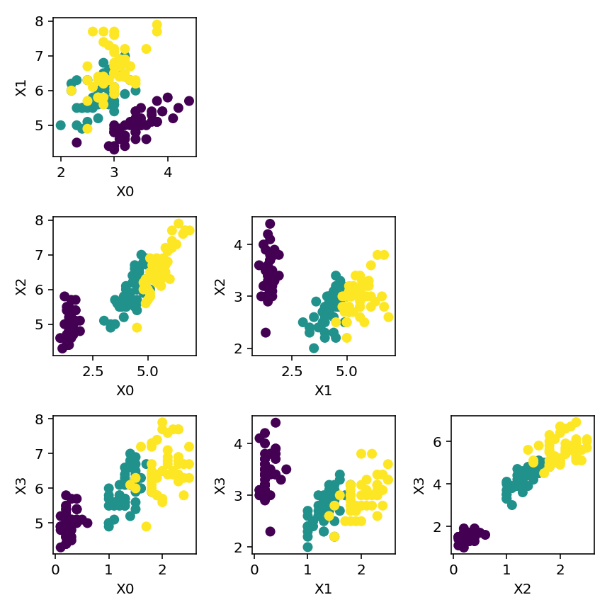 You can use
 plt.tight_layout() to adjust the space between subplots.
c) Make a quiver plot, representing sepal data by position, petal data by arrows, and flower type by arrow color.
d) Make a 3D scatter plot of the sepal and petal data, with the 4th column represented by marker size.
3) Surface plots#
a) Draw a wavy surface (not just a sine curve extended in the 3rd dimension).
b) Draw the surface of a (half) cylinder.
Note that the mesh grid does not need to be square.
A half cylinder (0 <= theta <= pi), using a square mesh grid:
A full cylinder (0 <= theta < 2pi), using a cylindrical mesh grid:
c) Draw the surface of a sphere.