2. Visualization: Exercise Solutions

import numpy as np
import matplotlib.pyplot as plt
%matplotlib inline

1) Plotting curves

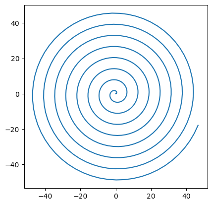
a) Draw a spiral.

t = np.arange(0, 50, 0.1)
x = t*np.cos(t)
y = t*np.sin(t)
plt.plot(x, y)
plt.axis('square')

(-51.77109696676726, 51.90297525317834, -53.41177025379329, 50.26230196615231)

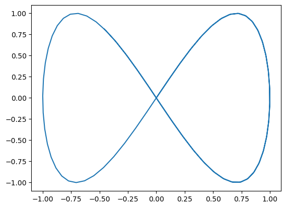
b) Draw a “\(\infty\)” shape.

t = np.arange(0,10,0.1)
x = np.sin(t)
y = np.sin(2*t)
plt.plot(x,y)

[<matplotlib.lines.Line2D at 0x107ad7b90>]

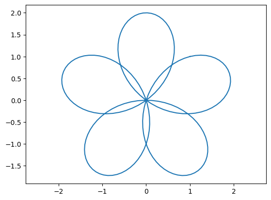
c) Draw a “flower-like” shape.

t = np.linspace(0, 2*np.pi, 200)
x = np.cos(t) + np.sin(4*t)
y = np.sin(t) + np.cos(4*t)
plt.plot(x, y)
plt.axis('equal')

(-2.1205669965972866,
 2.120318849193128,
 -1.9077538771970324,
 2.1855287366497285)

2) Scatter plots

Let us take the famous iris data set.
First four columns are:

• SepalLength, SepalWidth, PetalLength, PetalWidth

The last column is the flower type:

• 1:Setosa, 2:Versicolor, 3:Virginica

!head data/iris.txt

5.1,3.5,1.4,0.2,1
4.9,3.0,1.4,0.2,1
4.7,3.2,1.3,0.2,1
4.6,3.1,1.5,0.2,1
5.0,3.6,1.4,0.2,1
5.4,3.9,1.7,0.4,1
4.6,3.4,1.4,0.3,1
5.0,3.4,1.5,0.2,1
4.4,2.9,1.4,0.2,1
4.9,3.1,1.5,0.1,1

First, we’ll read the data set from a text file.

X = np.loadtxt('data/iris.txt', delimiter=',')
print(X.shape, X)

(150, 5) [[5.1 3.5 1.4 0.2 1. ]
 [4.9 3.  1.4 0.2 1. ]
 [4.7 3.2 1.3 0.2 1. ]
 [4.6 3.1 1.5 0.2 1. ]
 [5.  3.6 1.4 0.2 1. ]
 [5.4 3.9 1.7 0.4 1. ]
 [4.6 3.4 1.4 0.3 1. ]
 [5.  3.4 1.5 0.2 1. ]
 [4.4 2.9 1.4 0.2 1. ]
 [4.9 3.1 1.5 0.1 1. ]
 [5.4 3.7 1.5 0.2 1. ]
 [4.8 3.4 1.6 0.2 1. ]
 [4.8 3.  1.4 0.1 1. ]
 [4.3 3.  1.1 0.1 1. ]
 [5.8 4.  1.2 0.2 1. ]
 [5.7 4.4 1.5 0.4 1. ]
 [5.4 3.9 1.3 0.4 1. ]
 [5.1 3.5 1.4 0.3 1. ]
 [5.7 3.8 1.7 0.3 1. ]
 [5.1 3.8 1.5 0.3 1. ]
 [5.4 3.4 1.7 0.2 1. ]
 [5.1 3.7 1.5 0.4 1. ]
 [4.6 3.6 1.  0.2 1. ]
 [5.1 3.3 1.7 0.5 1. ]
 [4.8 3.4 1.9 0.2 1. ]
 [5.  3.  1.6 0.2 1. ]
 [5.  3.4 1.6 0.4 1. ]
 [5.2 3.5 1.5 0.2 1. ]
 [5.2 3.4 1.4 0.2 1. ]
 [4.7 3.2 1.6 0.2 1. ]
 [4.8 3.1 1.6 0.2 1. ]
 [5.4 3.4 1.5 0.4 1. ]
 [5.2 4.1 1.5 0.1 1. ]
 [5.5 4.2 1.4 0.2 1. ]
 [4.9 3.1 1.5 0.1 1. ]
 [5.  3.2 1.2 0.2 1. ]
 [5.5 3.5 1.3 0.2 1. ]
 [4.9 3.1 1.5 0.1 1. ]
 [4.4 3.  1.3 0.2 1. ]
 [5.1 3.4 1.5 0.2 1. ]
 [5.  3.5 1.3 0.3 1. ]
 [4.5 2.3 1.3 0.3 1. ]
 [4.4 3.2 1.3 0.2 1. ]
 [5.  3.5 1.6 0.6 1. ]
 [5.1 3.8 1.9 0.4 1. ]
 [4.8 3.  1.4 0.3 1. ]
 [5.1 3.8 1.6 0.2 1. ]
 [4.6 3.2 1.4 0.2 1. ]
 [5.3 3.7 1.5 0.2 1. ]
 [5.  3.3 1.4 0.2 1. ]
 [7.  3.2 4.7 1.4 2. ]
 [6.4 3.2 4.5 1.5 2. ]
 [6.9 3.1 4.9 1.5 2. ]
 [5.5 2.3 4.  1.3 2. ]
 [6.5 2.8 4.6 1.5 2. ]
 [5.7 2.8 4.5 1.3 2. ]
 [6.3 3.3 4.7 1.6 2. ]
 [4.9 2.4 3.3 1.  2. ]
 [6.6 2.9 4.6 1.3 2. ]
 [5.2 2.7 3.9 1.4 2. ]
 [5.  2.  3.5 1.  2. ]
 [5.9 3.  4.2 1.5 2. ]
 [6.  2.2 4.  1.  2. ]
 [6.1 2.9 4.7 1.4 2. ]
 [5.6 2.9 3.6 1.3 2. ]
 [6.7 3.1 4.4 1.4 2. ]
 [5.6 3.  4.5 1.5 2. ]
 [5.8 2.7 4.1 1.  2. ]
 [6.2 2.2 4.5 1.5 2. ]
 [5.6 2.5 3.9 1.1 2. ]
 [5.9 3.2 4.8 1.8 2. ]
 [6.1 2.8 4.  1.3 2. ]
 [6.3 2.5 4.9 1.5 2. ]
 [6.1 2.8 4.7 1.2 2. ]
 [6.4 2.9 4.3 1.3 2. ]
 [6.6 3.  4.4 1.4 2. ]
 [6.8 2.8 4.8 1.4 2. ]
 [6.7 3.  5.  1.7 2. ]
 [6.  2.9 4.5 1.5 2. ]
 [5.7 2.6 3.5 1.  2. ]
 [5.5 2.4 3.8 1.1 2. ]
 [5.5 2.4 3.7 1.  2. ]
 [5.8 2.7 3.9 1.2 2. ]
 [6.  2.7 5.1 1.6 2. ]
 [5.4 3.  4.5 1.5 2. ]
 [6.  3.4 4.5 1.6 2. ]
 [6.7 3.1 4.7 1.5 2. ]
 [6.3 2.3 4.4 1.3 2. ]
 [5.6 3.  4.1 1.3 2. ]
 [5.5 2.5 4.  1.3 2. ]
 [5.5 2.6 4.4 1.2 2. ]
 [6.1 3.  4.6 1.4 2. ]
 [5.8 2.6 4.  1.2 2. ]
 [5.  2.3 3.3 1.  2. ]
 [5.6 2.7 4.2 1.3 2. ]
 [5.7 3.  4.2 1.2 2. ]
 [5.7 2.9 4.2 1.3 2. ]
 [6.2 2.9 4.3 1.3 2. ]
 [5.1 2.5 3.  1.1 2. ]
 [5.7 2.8 4.1 1.3 2. ]
 [6.3 3.3 6.  2.5 3. ]
 [5.8 2.7 5.1 1.9 3. ]
 [7.1 3.  5.9 2.1 3. ]
 [6.3 2.9 5.6 1.8 3. ]
 [6.5 3.  5.8 2.2 3. ]
 [7.6 3.  6.6 2.1 3. ]
 [4.9 2.5 4.5 1.7 3. ]
 [7.3 2.9 6.3 1.8 3. ]
 [6.7 2.5 5.8 1.8 3. ]
 [7.2 3.6 6.1 2.5 3. ]
 [6.5 3.2 5.1 2.  3. ]
 [6.4 2.7 5.3 1.9 3. ]
 [6.8 3.  5.5 2.1 3. ]
 [5.7 2.5 5.  2.  3. ]
 [5.8 2.8 5.1 2.4 3. ]
 [6.4 3.2 5.3 2.3 3. ]
 [6.5 3.  5.5 1.8 3. ]
 [7.7 3.8 6.7 2.2 3. ]
 [7.7 2.6 6.9 2.3 3. ]
 [6.  2.2 5.  1.5 3. ]
 [6.9 3.2 5.7 2.3 3. ]
 [5.6 2.8 4.9 2.  3. ]
 [7.7 2.8 6.7 2.  3. ]
 [6.3 2.7 4.9 1.8 3. ]
 [6.7 3.3 5.7 2.1 3. ]
 [7.2 3.2 6.  1.8 3. ]
 [6.2 2.8 4.8 1.8 3. ]
 [6.1 3.  4.9 1.8 3. ]
 [6.4 2.8 5.6 2.1 3. ]
 [7.2 3.  5.8 1.6 3. ]
 [7.4 2.8 6.1 1.9 3. ]
 [7.9 3.8 6.4 2.  3. ]
 [6.4 2.8 5.6 2.2 3. ]
 [6.3 2.8 5.1 1.5 3. ]
 [6.1 2.6 5.6 1.4 3. ]
 [7.7 3.  6.1 2.3 3. ]
 [6.3 3.4 5.6 2.4 3. ]
 [6.4 3.1 5.5 1.8 3. ]
 [6.  3.  4.8 1.8 3. ]
 [6.9 3.1 5.4 2.1 3. ]
 [6.7 3.1 5.6 2.4 3. ]
 [6.9 3.1 5.1 2.3 3. ]
 [5.8 2.7 5.1 1.9 3. ]
 [6.8 3.2 5.9 2.3 3. ]
 [6.7 3.3 5.7 2.5 3. ]
 [6.7 3.  5.2 2.3 3. ]
 [6.3 2.5 5.  1.9 3. ]
 [6.5 3.  5.2 2.  3. ]
 [6.2 3.4 5.4 2.3 3. ]
 [5.9 3.  5.1 1.8 3. ]]

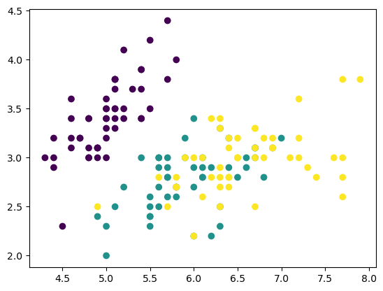
a) Make a scatter plot of the first two columns, with a distinct marker color for each flower type.

plt.scatter(X[:,0], X[:,1], c=X[:,-1])

<matplotlib.collections.PathCollection at 0x107a44e90>

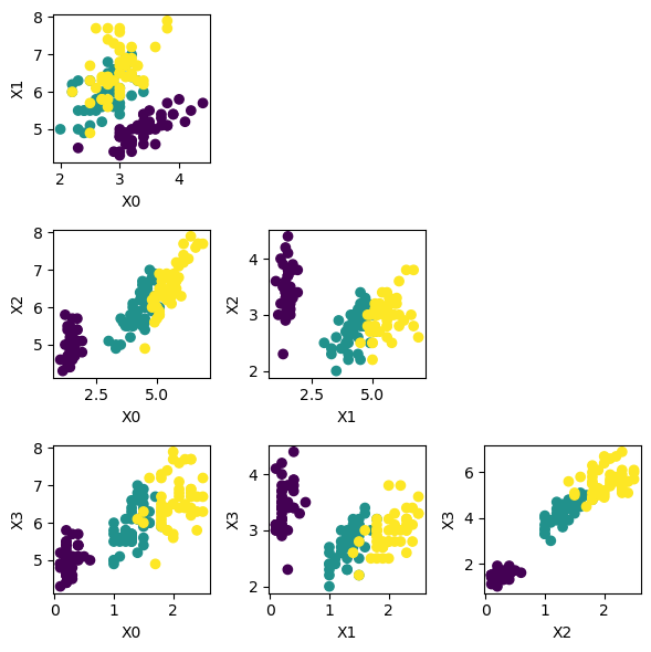
b) Create a matrix of pair-wise scatter plots like this:

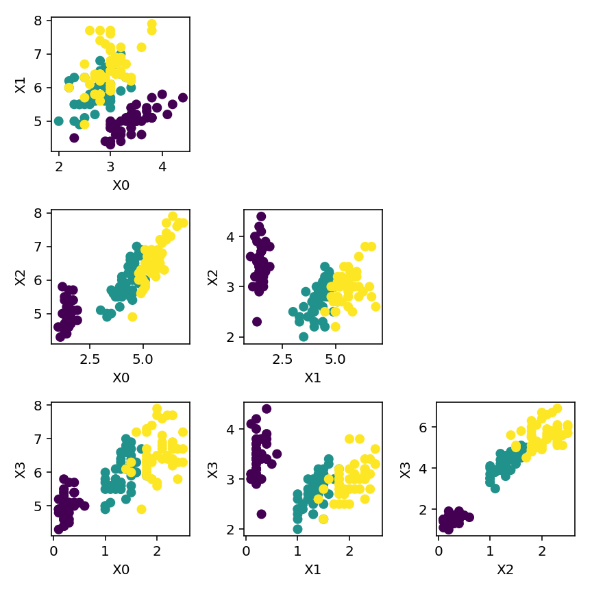
plt.figure(figsize=(6, 6))  # a bit larger area
d = 4  # data dimension
for i in range(1, d):  # rows: X1 to Xd
    for j in range(d-1):  # columns: X0 to Xd-1
        if j < i:
            plt.subplot(d-1, d-1, (i-1)*(d-1) + j+1)
            plt.scatter(X[:,i], X[:,j], c=X[:,-1])
            plt.ylabel('X{0}'.format(i))
            plt.xlabel('X{0}'.format(j))
plt.tight_layout()  # adjust the space between subplots

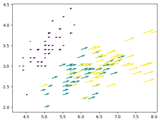
c) Make a quiver plot, representing sepal data by position, petal data by arrows, and flower type by arrow color.

plt.quiver(X[:,0], X[:,1], X[:,2], X[:,3], X[:,-1])

<matplotlib.quiver.Quiver at 0x107de9f10>

%matplotlib notebook

d) Make a 3D scatter plot of the sepal and petal data, with the 4th column represented by marker size.

fig = plt.figure()
ax = fig.add_subplot(projection='3d')
ax.scatter(X[:,0], X[:,1], X[:,2], s=20*X[:,3], c=X[:,-1])

<mpl_toolkits.mplot3d.art3d.Path3DCollection at 0x107e30710>

3) Surface plots

a) Draw a wavy surface (not just a sine curve extended in the 3rd dimension).

x = np.linspace(-10, 10, 50)
y = np.linspace(-10, 10, 50)
X, Y = np.meshgrid(x, y)
R = np.sqrt(X**2 + Y**2)
Z = np.sin(R)/R
fig = plt.figure()
ax = fig.add_subplot(projection='3d')
ax.plot_surface(X, Y, Z, cmap='viridis')

<mpl_toolkits.mplot3d.art3d.Poly3DCollection at 0x107a6a780>

b) Draw the surface of a (half) cylinder.
Note that the mesh grid does not need to be square.

A half cylinder (0 <= theta <= pi), using a square mesh grid:

r = 1
x = np.linspace(-r, r, 50)
y = np.linspace(-r, r, 50)
X, Y = np.meshgrid(x, y)
Z = np.sqrt(r**2 - Y**2)
fig = plt.figure()
ax = fig.add_subplot(projection='3d')
ax.plot_surface(X, Y, Z)

<mpl_toolkits.mplot3d.art3d.Poly3DCollection at 0x107d44770>

A full cylinder (0 <= theta < 2pi), using a cylindrical mesh grid:

r = 1
x = np.linspace(-r, r, 50)
th = np.linspace(0, 2*np.pi, 50)
X, Th = np.meshgrid(x, th)
Y = r*np.cos(Th)
Z = r*np.sin(Th)
fig = plt.figure()
ax = fig.add_subplot(projection='3d')
ax.plot_surface(X, Y, Z)

<mpl_toolkits.mplot3d.art3d.Poly3DCollection at 0x107e02060>

c) Draw the surface of a sphere.

r = 1
th = np.linspace(-np.pi/2, np.pi/2, 50)  # latitude
ph = np.linspace(-np.pi, np.pi, 50)  # longitude
Th, Ph = np.meshgrid(th, ph)
X = r*np.cos(Th)*np.cos(Ph)
Y = r*np.cos(Th)*np.sin(Ph)
Z = r*np.sin(Th)
fig = plt.figure()
ax = fig.add_subplot(projection='3d')
ax.plot_surface(X, Y, Z)
ax.set_box_aspect((1,1,1))