9. Stochastic Methods#
Some computations involve random numbers, such as simulating stochastic processes or searching in a high dimension space.
References:
Christopher M. Bishop: Pattern Recognition and Machine Learning, Chapter 11: Sampling methods. Springer, 2006.
Jun S. Liu: Monte Carlo Strategies in Scientific Computing. Springer, 2004.
import numpy as np
import matplotlib.pyplot as plt
%matplotlib inline
Random Numbers#
How can we generate random numbers from deterministic digital computers? They are, of course, pseudo random numbers.
The classic way of generating pseudo random numbers is Linear Congruent Method using a sequential dynimcs:
Below is what was long used in the Unix system.
def lcm(n=1, seed=-1726662223):
    """Random integers <2**31 by linear congruent method"""
    a = 1103515245
    b = 12345
    c = 0x7fffffff  # 2**31 - 1
    x = np.zeros(n+1, dtype=int)
    x[0] = seed
    for i in range(n):
        x[i+1] = (a*x[i] + b) & c  # bit-wise and
    return(x[1:])
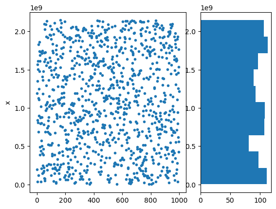
x = lcm(1000)
plt.subplot(1, 3, (1,2))
plt.plot(x, '.')
plt.ylabel('x')
plt.subplot(1, 3, 3)
plt.hist(x, orientation='horizontal');
A common problem with LCM is that lower digits can fall in simple cycles.
x[:100]%4
array([2, 3, 0, 1, 2, 3, 0, 1, 2, 3, 0, 1, 2, 3, 0, 1, 2, 3, 0, 1, 2, 3,
       0, 1, 2, 3, 0, 1, 2, 3, 0, 1, 2, 3, 0, 1, 2, 3, 0, 1, 2, 3, 0, 1,
       2, 3, 0, 1, 2, 3, 0, 1, 2, 3, 0, 1, 2, 3, 0, 1, 2, 3, 0, 1, 2, 3,
       0, 1, 2, 3, 0, 1, 2, 3, 0, 1, 2, 3, 0, 1, 2, 3, 0, 1, 2, 3, 0, 1,
       2, 3, 0, 1, 2, 3, 0, 1, 2, 3, 0, 1])
Also the samples can form crystal-like structure when consecutive numbers are taken as a vector.
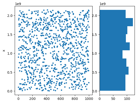
numpy.random uses an advanced method called Mersenne Twister which overcomes these problems.
x = np.random.randint(2**31, size=1000)
plt.subplot(1, 3, (1,2))
plt.plot(x, '.')
plt.ylabel('x')
plt.subplot(1, 3, 3)
plt.hist(x, orientation='horizontal');
x[:100]%4
array([0, 1, 0, 2, 0, 0, 1, 0, 2, 0, 2, 0, 2, 1, 3, 3, 3, 1, 0, 1, 2, 2,
       1, 1, 0, 0, 1, 0, 0, 2, 3, 1, 1, 0, 3, 2, 1, 2, 2, 1, 2, 0, 1, 3,
       2, 1, 1, 3, 0, 1, 2, 3, 3, 2, 2, 1, 2, 2, 3, 1, 1, 0, 2, 1, 3, 2,
       0, 1, 0, 3, 1, 3, 0, 2, 2, 2, 3, 3, 2, 3, 2, 1, 1, 1, 1, 0, 2, 0,
       0, 2, 0, 3, 1, 1, 1, 3, 0, 2, 3, 2])
Integrating area/volume#
Uniform random numbers can be used to approximate integration
by uniform samples \(x_i\) in a volume \(V\)
For example, let us evaluate a volume of a sphere.
# Sphere in 3D
def sphere(x):
    """height of a half sphere"""
    h2 = 1 - x[0]**2 - x[1]**2
    return np.sqrt((h2>0)*h2)
m = 10000
x = np.random.random((2, m)) # one quadrant
v = np.sum(sphere(x))/m
print(8*v)
print(4/3*np.pi)
4.195754621869497
4.1887902047863905
Let us evaluate the volume of n-dimension sphere, which is supposed to be
from scipy.special import gamma
# n-dimensional sphere
def nsphere(x):
    """height of a half sphere in n-dim"""
    h2 = 1 - np.sum(x**2, axis=0)
    return np.sqrt((h2>0)*h2)
m = 10000
for n in range(2,20):
    x = np.random.random((n-1, m)) # one quadrant
    v = np.sum(nsphere(x))/m
    print(n, 2**n*v, np.pi**(n/2)/gamma(n/2+1))
2 3.158124715415353 3.141592653589793
3 4.169849266923301 4.188790204786391
4 4.992167148448152 4.934802200544679
5 5.092332342303803 5.263789013914324
6 5.309607266535629 5.167712780049969
7 4.394979816274948 4.724765970331401
8 3.851599880914358 4.058712126416768
9 3.091119557136502 3.2985089027387064
10 2.0518403094303954 2.550164039877345
11 1.5074553893648002 1.8841038793898999
12 1.948270254662379 1.3352627688545893
13 0.739601544093307 0.9106287547832829
14 1.7064203392589348 0.5992645293207919
15 0.0 0.38144328082330436
16 0.0 0.23533063035889312
17 0.0 0.140981106917139
18 0.0 0.08214588661112819
19 0.0 0.04662160103008853
Non-uniform Distributions#
How can we generate samples following a non-uniform distribution \(p(x)\)?
If the cumulative density function
is known, we can map uniformly distributed samples \(y_i\in[0,1]\) to \(x_i = f^{-1}(y_i)\).
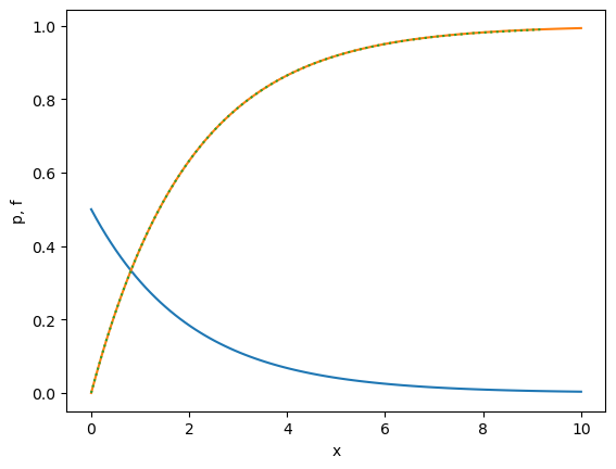
Exponential distribution#
# Exponential distribution in [0,infinity)
def p_exp(x, mu=1):
    """density function of exponential distribution"""
    return np.exp(-x/mu)/mu

def f_exp(x, mu=1):
    """cumulative density function of exponential distribution"""
    return 1 - np.exp(-x/mu)

def finv_exp(y, mu=1):
    """inverse of cumulative density function of exponential distribution"""
    return -mu*np.log(1 - y)
x = np.linspace(0, 10, 100)
plt.plot(x, p_exp(x, 2))
plt.plot(x, f_exp(x, 2))
y = np.arange(0, 1, 0.01)
plt.plot(finv_exp(y, 2), y, ':')
plt.xlabel('x'); plt.ylabel('p, f');
def x_exp(n=1, mu=1):
    """sample from exponential distribution"""
    ys = np.random.random(n)  # uniform in [0,1]
    return finv_exp(ys, mu)
x_exp(10, 2)
array([1.98917361, 0.22379092, 0.40570992, 1.73172977, 2.8249073 ,
       0.97152565, 3.17584295, 0.1176832 , 2.34714779, 4.69828058])
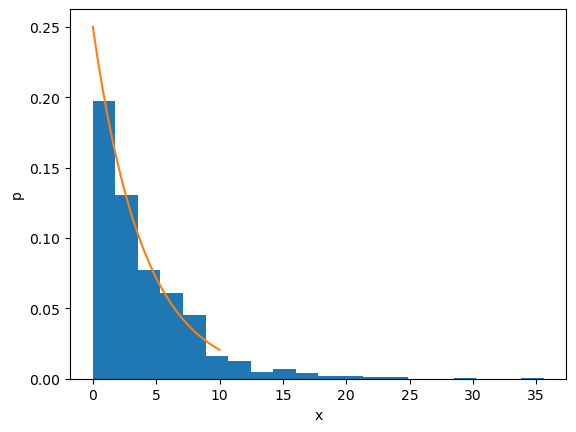
xs = x_exp(1000, 4)
plt.hist(xs, bins=20, density=True)
plt.plot(x, p_exp(x, 4))
plt.xlabel('x'); plt.ylabel('p');
When a stochastic variable \(x\) following the distribution \(p(x)\) is transformed by \(y=g(x)\), the distribution of \(y\) is given by
where \(|\,|\) means the absolute value for a scalar derivative and the determinant for a Jacobian matrix.
Normal distribution#
A common way of generating a normal (Gaussian) distribution
is to consider a 2D normal distribution
For a polar coordinate tranformation
the Jacobian is
and its determinant is
Thus we have the relationship
By further transforming \(u=r^2\), from \(\frac{du}{dr}= 2r\), we have
Thus we can sample \(u\) by exponential distribution
and \(\theta\) by uniform distribution in \([0,2\pi)\), and then transform them to \(x_1\) and \(x_2\) to generate two samples following normal distribution.
This is known as Box-Muller method.
def box_muller(n=1):
    """Generate 2n gaussian samples"""
    u = x_exp(n, 2)
    r = np.sqrt(u)
    theta = 2*np.pi*np.random.random(n)
    x1 = r*np.cos(theta)
    x2 = r*np.sin(theta)
    return np.hstack((x1,x2))
box_muller(1)
array([ 0.00354795, -1.0042656 ])
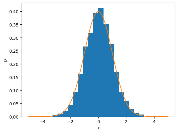
xs = box_muller(1000)
plt.hist(xs, bins=20, density=True)
# check how the histogram fits the pdf
x = np.linspace(-5, 5, 100)
px = np.exp(-x**2/2)/np.sqrt(2*np.pi)
plt.plot(x, px)
plt.xlabel('x'); plt.ylabel('p');
In practice, you can sample by the whole variety of distributions in numpy.random package, but it’s good to know the principle.
#help(np.random)
Rejection Sampling#
What can we do when transformations from uniform distribution is not available?
Let us find a proposal distribution \(q(x)\) for which samples are easily generated and covers the target distribution as \(p(x)\le cq(x)\) with a scaling constant \(c>0\).
Then take a sample from \(q(x)\) and accept it with probability \(\frac{p(x)}{cq(x)}\).
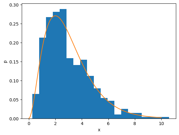
Gamma distribution#
Gamma distribution is an extension of exponential distribution defined as
with the shape parameter \(k>0\) and the scaling parameter \(\theta\).
\(\Gamma(k)\) is the gamma function, which is a generalization of factorial, \(\Gamma(k)=(k-1)!\) for an integer \(k\).
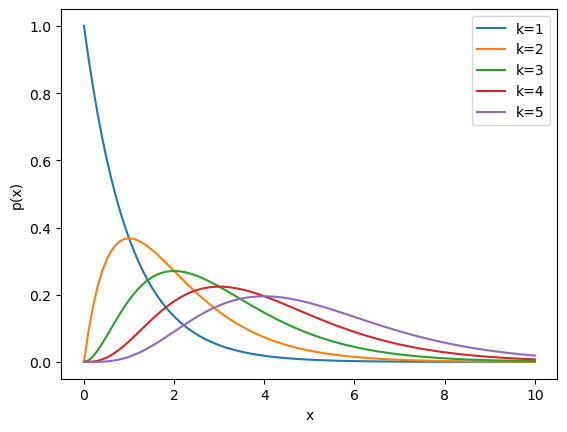
Let us generate samples from gamma distribution with integer \(k\) and \(\theta=1\).
def p_gamma(x, k=1):
    """gamma distribution with integer k"""
    return x**(k-1)*np.exp(-x)/np.prod(range(1,k))
x = np.linspace(0, 10, 100)
for k in range(1, 6):
    plt.plot(x, p_gamma(x, k), label='k={}'.format(k))
plt.xlabel('x'); plt.ylabel('p(x)'); plt.legend();
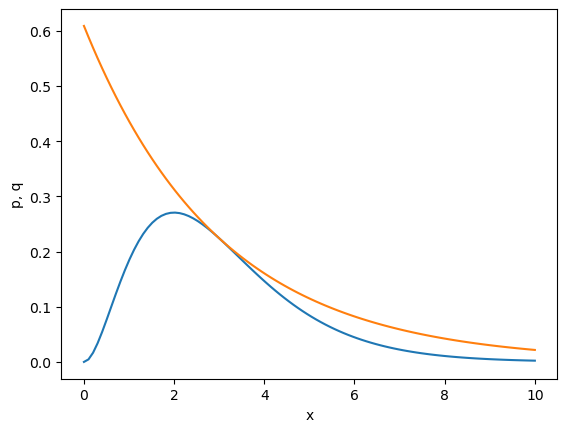
Consider the exponential distribution \(q(x;\mu)=\frac{1}{\mu}e^{-\frac{x}{\mu}}\) as the proposal distribution.
For
we set
and have
where \(\frac{p(x;k)}{q(x;\mu)}\) takes the maximum
By taking \(\mu=k\),
satisfies \(p(x)\le cq(x)\)
k = 3
c = (k**k)/np.prod(range(1,k))*np.exp(1-k)
#print(c)
x = np.linspace(0, 10, 100)
plt.plot(x, p_gamma(x, k))
plt.plot(x, c*p_exp(x, k))
plt.xlabel('x'); plt.ylabel('p, q');
def x_gamma(n=10, k=1):
    """sample from gamma distribution by rejection sampling"""
    c = (k**k)/np.prod(range(1,k))*np.exp(1-k)
    xe = x_exp(n, k)
    paccept = p_gamma(xe, k)/(c*p_exp(xe, k))
    accept = np.random.random(n)<paccept
    xg = xe[accept]  # rejection sampling
    #print("c =", c, "; acceptance rate =", len(xg)/n)
    return xg
k = 3
xs = x_gamma(1000, k)
print('accept:', len(xs))
plt.hist(xs, bins=20, density=True)
plt.plot(x, p_gamma(x, k))
plt.xlabel('x'); plt.ylabel('p');
accept: 538
Importance Sampling#
One probelm of rejection sampling is that we may end up rejecting many of the samples when we cannot find a good proposal distribution.
When the aim is not just to take samples from \(p(x)\) but to take the expectation of a function \(h(x)\) with respect to the distribution \(p(x)\)
we can use the ratio between the target and proposal distributions to better utilize the samples.
Mean and variance#
Let us consider taking the mean
and the variance
for the gamma distribution, which are known to be \(k\theta\) and \(k\theta^2\), respectively.
def mv_exp(n=1, mu=1):
    """mean and variance of exponential distribution"""
    x = x_exp(n, mu)
    mean = np.mean(x)
    var = np.var(x)
    return (mean, var)
mv_exp(1000, 3)
(2.9682255567705624, 9.367895293279625)
def mv_gamma(n=1, k=1):
    """mean and variance of gamma distribution by rejection sampling"""
    x = x_gamma(n, k)  # by rejection sampling
    mean = np.mean(x)
    var = np.var(x)
    return (mean, var)
mv_gamma(100, 3)
(3.2266054925420193, 2.9009214451170324)
def mv_gamma_is(n=1, k=1):
    """mean and variance of gamma distribution by importance sampling"""
    x = x_exp(n, k)  # sample by exponential distribution
    importance = p_gamma(x, k)/p_exp(x, k)
    mean = np.dot(importance, x)/n
    var = np.dot(importance, (x-mean)**2)/(n - 1)
    return (mean, var)
mv_gamma_is(1000, 3)
(2.978285147753999, 3.013995547532964)
Compare the variability of the estimate of the mean.
m = 100  # number of runs
n = 100  # number of samples
k = 3
means = np.zeros((m, 2))
for i in range(m):
    means[i,0], var = mv_gamma(n, k)
    means[i,1], var = mv_gamma_is(n, k)
print("RS: ", np.mean(means[:,0]), np.var(means[:,0]))
print("IS: ", np.mean(means[:,1]), np.var(means[:,1]))
RS:  2.998402287691978 0.05617207305635085
IS:  2.947997467572822 0.06777538309226606
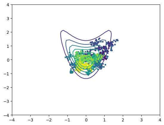
Markov Chain Monte Carlo (MCMC)#
What if we don’t know the right proposal distribution? We can take a nearby point of a previous sample as a candidate sample and keep it if the candidate’s probability is high. The method is callel Markov Chain Monte Carlo (MCMC) method and used practically for sampling from unknow distributions in high dimensional space.
Metropolis Sampling#
A simple example of MCMC is Metropolis sampling, which requires only unnormalized propability \(\tilde{p}(x)\propto p(x)\) of samples for relative comparison.
A new candidate \(x^*\) is generated by a symmetric proposal distribution \(q(x^*|x_k)=q(x_k|x^*)\), such as a gaussian distribution, and acctepted with the probability of
def metropolis(p, x0, sig=0.1, m=1000):
    """metropolis: Metropolis sampling
    p:unnormalized probability, x0:initial point,
    sif:sd of proposal distribution, m:number of sampling"""
    n = len(x0)  # dimension
    p0 = p(x0)
    x = []
    for i in range(m):
        x1 = x0 + sig*np.random.randn(n)
        p1 = p(x1)
        pacc = min(1, p1/p0)
        if np.random.rand()<pacc:
            x.append(x1)
            x0 = x1
            p0 = p1
    return np.array(x)
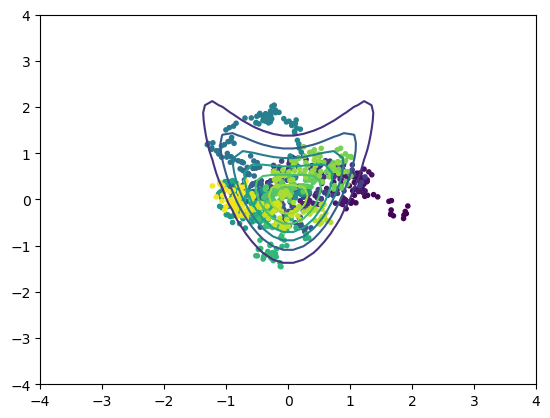
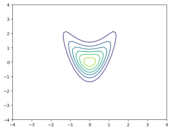
def croissant(x):
    """croissant-like distribution in 2D"""
    return np.exp(-x[0]**2 - (x[1]-x[0]**2)**2)
r = 4  # plot rage
x = np.linspace(-r, r)
X, Y = np.meshgrid(x, x)
Z = croissant(np.array([X,Y]))
plt.contour(X, Y, Z);
x = metropolis(croissant, [0,0])
s = len(x); print(s)
plt.contour(X, Y, Z)
plt.scatter(x[:,0], x[:,1], c=np.arange(s), marker='.');
915
x = metropolis(croissant, [2,0], sig=0.1, m=1000)
s = len(x); print(s)
plt.contour(X, Y, Z)
plt.scatter(x[:,0], x[:,1], c=np.arange(s), marker='.');
907