8. Optimization#
Research involves lots of parmeter tuing. When there are just a few paramters, we often tune them by hand using our intuition or run a grid search. But when the number of parameters is large or it is difficult to get any intuition, we need a systematic method for optimization.
Optimization is in general considered as minimization or maximization of a certain objective function \(f(x)\) where \(x\) is a parameter vector. There are different cases:
If the mathematical form of the objective function \(f(x)\) is known:
put derivatieves \(\frac{\partial f(x)}{\partial x}=0\) and solve for \(x\).
check the signs of second order derivatives \(\frac{\partial^2 f(x)}{\partial x^2}\)
if all positive, that is a minimum
if all negative, that is a maximum
if mixed, that is a saddle point
If analytic solution of \(\frac{\partial f(x)}{\partial x}=0\) is hard to derive:
gradient descent/ascent
Newton-Raphson method
conjugate gradient method
If the derivatives of \(f(x)\) is hard to derive:
genetic/evolutionary algorithms
sampling methods (next week)
If \(f(x)\) needs to be optimized under constraints, such as \(g(x)\le 0\) or \(h(x)=0\):
penalty function
Lagrange multiplyer method
linear programming if \(f(x)\) is linear
quadratic programming if \(f(x)\) is quadratic
References:
Jan A. Snyman: Practical Mathematial Optimization. Springer, 2005.
SciPy Lecture Notes: 1.5.5 Optimization and fit
import numpy as np
import matplotlib.pyplot as plt
%matplotlib inline
from mpl_toolkits.mplot3d import Axes3D
Example#
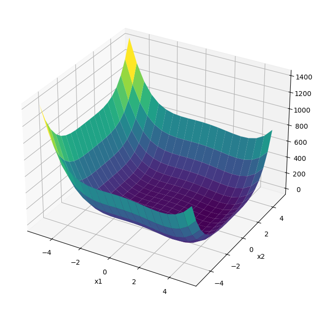
For the sake of visualization, consider a function in 2D space \(x=(x_1,x_2)\)
The gradient is
By putting \(\nabla f(x)=0\), we have
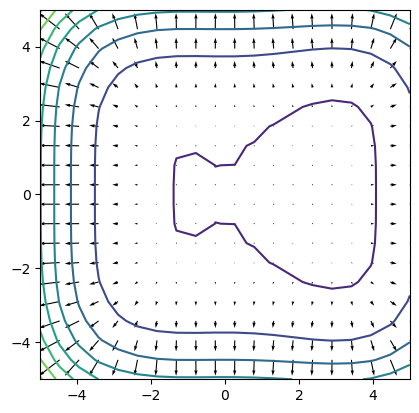
so there are three points with zero gradient: \((-1,0)\), \((0,0)\), \((3,0)\).
You can check the second-order derivative, or Hessian, to see if they are a minimum, a saddle point, or a maximum.
As \(\frac{\partial^2 f(x)}{\partial x_1^2}\) is positive for \(x_1=-1\) and \(x_1=3\) and negative for \(x_1=0\), \((-1,0)\) and \((3,0)\) are minima and \((0,0)\) is a saddle point.
Let us visualize this.
def dips(x):
    """a function to minimize"""
    f = x[0]**4 - 8/3*x[0]**3 - 6*x[0]**2 + x[1]**4
    return(f)

def dips_grad(x):
    """gradient of dips(x)"""
    df1 = 4*x[0]**3 - 8*x[0]**2 - 12*x[0]
    df2 = 4*x[1]**3
    return(np.array([df1, df2]))

def dips_hess(x):
    """hessian of dips(x)"""
    df11 = 12*x[0]**2 - 16*x[0] - 12
    df12 = 0
    df22 = 12*x[1]**2
    return(np.array([[df11, df12], [df12, df22]]))
x1, x2 = np.meshgrid(np.linspace(-5, 5, 20), np.linspace(-5, 5, 20))
fx = dips([x1, x2])
# 3D plot
fig = plt.figure(figsize=(8, 8))
ax = fig.add_subplot(111, projection='3d')
ax.plot_surface(x1, x2, fx, cmap='viridis')
ax.set_xlabel('x1')
ax.set_ylabel('x2')
Text(0.5, 0.5, 'x2')
plt.contour(x1, x2, fx)
dfx = dips_grad([x1, x2])
plt.quiver(x1, x2, dfx[0], dfx[1])
plt.axis('square')
(np.float64(-5.0), np.float64(5.0), np.float64(-5.0), np.float64(5.0))
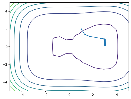
Gradient Descent/Ascent#
Gradient descent/ascent is the most basic method of min/maximization of a function using its gradient.
From an initial state \(x_0\) and a coefficient \(\eta>0\), repeat
for minimization.
def grad_descent(f, df, x0, eta=0.01, eps=1e-6, imax=1000):
    """Gradient descent"""
    xh = np.zeros((imax+1, len(np.ravel([x0]))))  # history
    xh[0] = x0
    f0 = f(x0)  # initialtization
    for i in range(imax):
        x1 = x0 - eta*df(x0)
        f1 = f(x1)
        # print(x1, f1)
        xh[i+1] = x1
        if(f1 <= f0 and f1 > f0 - eps):  # small decrease
            return(x1, f1, xh[:i+2])
        x0 = x1
        f0 = f1
    print("Failed to converge in ", imax, " iterations.")
    return(x1, f1, xh)
xmin, fmin, xhist = grad_descent(dips, dips_grad, [1,2], 0.02)
print(xmin, fmin)
plt.contour(x1, x2, fx)
plt.plot(xhist[:,0], xhist[:,1], '.-')
#plt.axis([1, 4, -1, 3])
[3. 0.1206838] -44.99978787303231
[<matplotlib.lines.Line2D at 0x11cf825d0>]
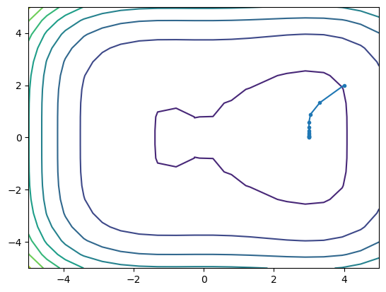
Newton-Raphson Method#
A problem with the gradient descence/ascent is the choice of the coefficient \(\eta\). If the second-order derivative, called the Hessian,
is available, we can use the Newton method to find the solution for
by repeating
This is called Newton-Raphson method. It works efficiently when the Hessian is positive definite (\(f(x)\) is like a parabolla), but can be unstable when the Hessian has a negative eigenvalue (near the saddle point).
def newton_raphson(f, df, d2f, x0, eps=1e-6, imax=1000):
    """Newton-Raphson method"""
    xh = np.zeros((imax+1, len(np.ravel([x0]))))  # history
    xh[0] = x0
    f0 = f(x0)  # initialtization
    for i in range(imax):
        x1 = x0 - np.linalg.inv(d2f(x0)) @ df(x0)
        f1 = f(x1)
        #print(x1, f1)
        xh[i+1] = x1
        if( f1 <= f0 and f1 > f0 - eps):  # decreasing little
            return(x1, f1, xh[:i+2])
        x0 = x1
        f0 = f1
    print("Failed to converge in ", imax, " iterations.")
    return(x1, f1, xh)
xmin, fmin, xhist = newton_raphson(dips, dips_grad, dips_hess, [4,2])
print(xmin, fmin)
plt.contour(x1, x2, fx)
plt.plot(xhist[:,0], xhist[:,1], '.-')
#plt.axis([1, 4, -1, 3])
[3. 0.01541469] -44.999999943540175
[<matplotlib.lines.Line2D at 0x11cfcf750>]
scipy.optimize#
To address those issues, advanced optimization algorithms have been developed and implemented in scipy.optimize package.
from scipy.optimize import minimize
The default method for unconstrained minimization is ‘BFGS’ (Broyden-Fletcher-Goldfarb-Shanno) method, a variant of gradient descent.
result = minimize(dips, [-1,2], jac=dips_grad, options={'disp': True})
print( result.x, result.fun)
Optimization terminated successfully.
         Current function value: -2.333333
         Iterations: 17
         Function evaluations: 18
         Gradient evaluations: 18
[-1.          0.01205015] -2.3333333122484903
If the gradient function is not specified, it is estimated by finite difference method.
result = minimize(dips, [2,2], options={'disp': True})
print( result.x, result.fun)
Optimization terminated successfully.
         Current function value: -45.000000
         Iterations: 19
         Function evaluations: 63
         Gradient evaluations: 21
[3.00000005 0.01058703] -44.999999987436844
‘Newton-CG’ (Newton-Conjugate-Gradient) is a variant of Newton-Raphson method using linear search in a conjugate direction.
result = minimize(dips, [2,2], method='Newton-CG',
          jac=dips_grad, hess=dips_hess, options={'disp': True})
print( result.x, result.fun)
Optimization terminated successfully.
         Current function value: -45.000000
         Iterations: 16
         Function evaluations: 17
         Gradient evaluations: 17
         Hessian evaluations: 16
[3.        0.0065082] -44.999999998205915
result
 message: Optimization terminated successfully.
 success: True
  status: 0
     fun: -44.999999998205915
       x: [ 3.000e+00  6.508e-03]
     nit: 16
     jac: [ 0.000e+00  1.103e-06]
    nfev: 17
    njev: 17
    nhev: 16
‘Nelder-Mead’ is a simplex method that uses a set of \(n+1\) points to estimate the gradient and select a new point by flipping the simplex.
note that it is totally different from the simplex method for linear programming.
result = minimize(dips, [2,2], method='Nelder-Mead', options={'disp': True})
print( result.x, result.fun)
Optimization terminated successfully.
         Current function value: -45.000000
         Iterations: 60
         Function evaluations: 119
[ 3.00000000e+00 -1.83332383e-05] -45.00000000000001
Constrained Optimization#
Often we want to minimize/maximize \(f(x)\) under constraints on \(x\), e.g.
inequality constraints
equality constraints
Penalty function#
Define a function with penalty terms:
and increase \(\rho\) to a large value.
Lagrange multiplyer method#
For minimization of \(f(x)\) with equality constraints \(h_j(x)=0\), \((j=1,...,r)\), define a Lagrangian function
The necessary condition for a minimum is:
Scipy implements SLSQP (Sequential Least SQuares Programming) method. Constraints are defined in a sequence of dictionaries.
# h(x) = - x[0] + x[1] - 0.6 = 0
def h(x):
    return -x[0] + x[1] - 0.6
def h_grad(x):
    return np.array([-1, 1])
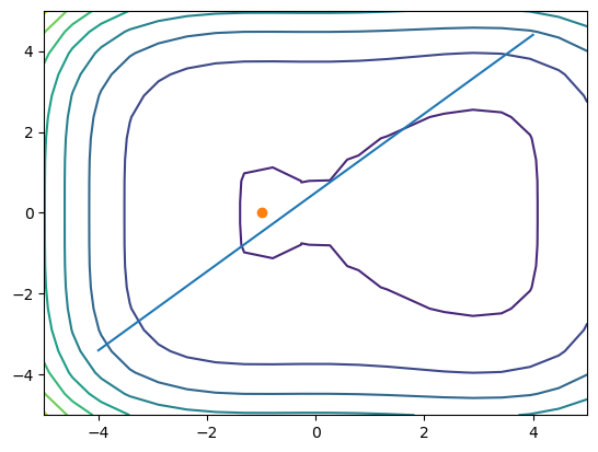
With equality constraint \(h(x)=0\).
cons = ({'type':'eq', 'fun':h, 'jac':h_grad})
result = minimize(dips, [1,-3], jac=dips_grad,
            method='SLSQP', constraints=cons, options={'disp': True})
print( result.x, result.fun)
plt.contour(x1, x2, fx)
plt.plot([-4,4], [-3.4,4.4])  # h(x) = 0
plt.plot(result.x[0], result.x[1], 'o')
Optimization terminated successfully    (Exit mode 0)
            Current function value: -1.1182207863637803
            Iterations: 9
            Function evaluations: 11
            Gradient evaluations: 9
[0.97276055 1.57276055] -1.1182207863637803
[<matplotlib.lines.Line2D at 0x11f95c2d0>]

With inequality constraint \(h(x)>0\).
cons = ({'type': 'ineq', 'fun': h, 'jac':h_grad})
result = minimize(dips, [1,-3], jac=dips_grad,
            method='SLSQP', constraints=cons, options={'disp': True})
print( result.x, result.fun)
plt.contour(x1, x2, fx)
plt.plot([-4,4], [-3.4,4.4])  # h(x) = 0
plt.plot(result.x[0], result.x[1], 'o')
Optimization terminated successfully    (Exit mode 0)
            Current function value: -2.3333329239019784
            Iterations: 16
            Function evaluations: 20
            Gradient evaluations: 16
[-1.00000016  0.02529561] -2.3333329239019784
[<matplotlib.lines.Line2D at 0x11f9b1450>]
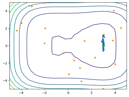
Genetic/Evolutionaly Algorithms#
For objective functions with many local minima/maxima, stochastic search methods are preferred. They are called genetic algorithm (GA) or evolutionay algorithm (EA), from an analogy with mutation and selection in genetic evolution.
def evol_min(f, x0, sigma=0.1, imax=100):
    """simple evolutionary algorithm
    f: function to be minimized
    x0: initial population (p*n)
    sigma: mutation size"""
    p, n = x0.shape  # population, dimension
    x1 = np.zeros((p, n))
    xh = np.zeros((imax, n))  # history
    for i in range(imax):
        f0 = f(x0.T)  # evaluate the current population
        fmin = min(f0)
        xmin = x0[np.argmin(f0)]
        #print(xmin, fmin)
        xh[i] = xmin  # record the best one
        # roulette selection
        fitness = max(f0) - f0  # how much better than the worst
        prob = fitness/sum(fitness)  # selection probability
        #print(prob)
        for j in range(p):  # pick a parent for j-th baby
            parent = np.searchsorted(np.cumsum(prob), np.random.random())
            x1[j] = x0[parent] + sigma*np.random.randn(n)
        x0 = x1
    return(xmin, fmin, xh)
x0 = np.random.rand(20, 2)*10 - 5
xmin, fmin, xhist = evol_min(dips, x0, 0.1)
print(xmin, fmin)
plt.contour(x1, x2, fx)
plt.plot(xhist[:,0], xhist[:,1], '.-')
plt.plot(x0[:,0], x0[:,1], '*')
plt.plot(xhist[-1,0], xhist[-1,1], 'o')
[ 3.178513 -0.18707914] -44.98351467942098
[<matplotlib.lines.Line2D at 0x11fa26710>]
For more advanced genetic/evolutionary algorithms, you can use deap package: DEAP