3. Vectors and Matrices: Exercise

Name:

\[ % Latex macros \newcommand{\mat}[1]{\begin{pmatrix} #1 \end{pmatrix}} \newcommand{\p}[2]{\frac{\partial #1}{\partial #2}} \newcommand{\b}[1]{\boldsymbol{#1}} \newcommand{\w}{\boldsymbol{w}} \newcommand{\x}{\boldsymbol{x}} \newcommand{\y}{\boldsymbol{y}} \]

import numpy as np
import matplotlib.pyplot as plt
%matplotlib inline

1) Determinant and eigenvalues

1. For a 2x2 matrix \(A = \left(\begin{array}{cc} a & b\\ c & d \end{array}\right)\), let us verify that \(\det A = ad - bc\) in the case graphically shown below (\(a, b, c, d\) are positive).

A = np.array([[4, 1], [2, 3]])
plt.plot([0, 1, 1, 0, 0], [0, 0, 1, 1, 0])
plt.plot([0, A[0,0]+A[0,1], A[0,0]+A[0,1], 0, 0], 
         [0, 0, A[1,0]+A[1,1], A[1,0]+A[1,1], 0])
plt.plot([A[0,0], A[0,0]+A[0,1], A[0,0]+A[0,1], A[0,0], A[0,0]], 
         [0, 0, A[1,0], A[1,0], 0])
plt.plot([0, A[0,1], A[0,1], 0, 0], 
         [A[1,1], A[1,1], A[1,0]+A[1,1], A[1,0]+A[1,1], A[1,1]])
plt.plot([0, A[0,0], A[0,0]+A[0,1], A[0,1], 0], 
         [0, A[1,0], A[1,0]+A[1,1], A[1,1], 0])
plt.axis('equal')
plt.text(A[0,0], A[1,0], '(a,c)')
plt.text(A[0,1], A[1,1], '(b,d)')
plt.text(A[0,0]+A[0,1], A[1,0]+A[1,1], '(a+b,c+d)');

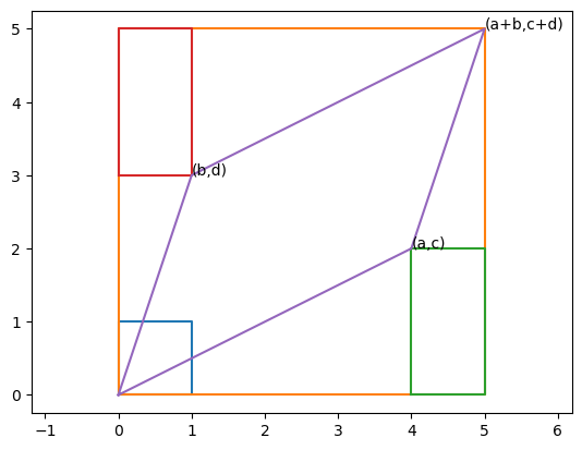
A unit square is transformed into a parallelogram. Its area \(S\) can be derived as follows:
Large rectangle: \( S_1 = (a+b)(c+d) \)
Small rectangle: \( S_2 = \)
Bottom/top triangle: \( S_3 = \)
Left/right triangle: \( S_4 = \)
Parallelogram: \( S = S_1 - ... \)

2. The determinant equals the product of all eigenvalues. Verify this numerically for multiple cases and explain intuitively why that should hold.

A = np.array(...
det = 
print('detA = ', det)
lam, V = 
print(np.product(lam))

  Cell In[3], line 1
    A = np.array(...
                ^
SyntaxError: '(' was never closed

The determinant represents …

The eigenvalues mean …

Therefore, …

2) Eigenvalues and matrix product

1. Make a random (or hand-designed) \(m\times m\) matrix \(A\). Compute its eigenvalues and eigenvectors. From a random (or your preferred) initial point \(\b{x}\), compute \(A\b{x}, A^2\b{x}, A^3\b{x},...\) and visualize the points. Then characterize the behavior of the points with respect the eigenvalues and eigenvectors.

2. Do the above with several different matrices

3) Principal component analysis

Read in the “digits” dataset, originally from sklearn.

data = np.loadtxt("data/digits_data.txt")
target = np.loadtxt("data/digits_target.txt", dtype='int64')
data.shape

The first ten samples look like these:

for i in range(10):
    plt.subplot(1,10,i+1)
    plt.imshow(data[i].reshape((8,8)))
    plt.title(target[i])

1. Compute the principal component vectors from all the digits and plot the eigenvalues from the largest to smallest.

2. Visualize the principal vectors as images.

3. Scatterplot the digits in the first two or three principal component space, with different colors/markers for digits.

4. Take a sample digit, decompose it into principal components, and reconstruct the digit from the first \(m\) components. See how the quality of reproduction depends on \(m\).