7. Partial Differential Equations

References:

• Svein Linge & Hans Petter Langtangen: Programming for Computations – Python. Springer (2016).

  • Chapter 5: Solving Partial Differential Equations

import numpy as np
import matplotlib.pyplot as plt
%matplotlib inline

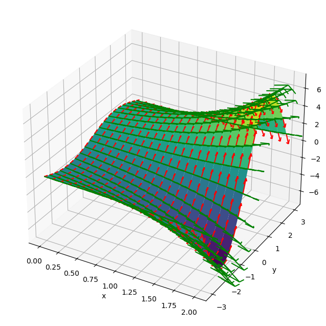
Partial derivative

For a function with multiple inputs \(f(x_1,...,x_n)\), a partial derivative is the derivative with respect to an input \(x_i\) while other inputs are held constant.

\[\frac{\partial f(x_1,...,x_n)}{\partial x_i} = \lim_{\Delta x \rightarrow 0} \frac{f(x_1,...,x_i+\Delta x,...,x_n) - f(x_1,...,x_i,...,x_n)}{\Delta x}\]

For example, for

\[ f(x,y) = e^{x} \sin y, \]

partial derivatives are

\[ \frac{\partial f(x,y)}{\partial x} = e^{x} \sin y \]

\[ \frac{\partial f(x,y)}{\partial y} = e^{x} \cos y \]

x, y = np.meshgrid(np.linspace(0, 2, 20), np.linspace(-3, 3, 20))
f = np.exp(x) * np.sin(y)
dfdx = np.exp(x) * np.sin(y)
dfdy = np.exp(x) * np.cos(y)
# 3D plot
fig = plt.figure(figsize=(8, 8))
ax = fig.add_subplot(projection='3d')
ax.plot_surface(x, y, f, cmap='viridis')
x0 = np.zeros_like(x)
x1 = np.ones_like(x)
ax.quiver(x, y, f, x1, x0, dfdx, color='g', length=0.2)
ax.quiver(x, y, f, x0, x1, dfdy, color='r', length=0.2)
plt.xlabel('x'); plt.ylabel('y');

Partial Differential Equation (PDE)

A partial differential equation (PDE) is an equation that includes partial derivatives

\[\frac{\partial f(x_1,...,x_n)}{\partial x_i}\]

of an unknown function \(f(x_1,...,x_n)\).

A typical case is a function in space and time \(y(x,t).\)

A simple example is the diffusion equation (or heat equation)

\[ \frac{\partial y(x,t)}{\partial t} = D \frac{\partial^2 y(x,t)}{\partial x^2} + g(y,x,t) \]

that describes the evolution of concentration (or temperature) \(y\) in space \(x\) and time \(t\) with input \(g(y,x,t)\) and the diffusion coefficient \(D\).

Analytic Solution of PDE

For a diffusion equation without input

\[ \frac{\partial y}{\partial t} = D \frac{\partial^2 y}{\partial x^2}, \]

the solution is given by separation of variables.

By assuming that the solution is a product of temporal and spatial components \(y(x,t) = u(t) v(x)\), the PDE becomes

\[ \frac{\partial u(t)}{\partial t} v(x)= D u(t) \frac{\partial^2 v(x)}{\partial x^2} \]

\[ \frac{1}{Du(t)}\frac{\partial u(t)}{\partial t} = \frac{1}{v(x)}\frac{\partial^2 v(x)}{\partial x^2} \]

For this equation to hold for any \(t\) and \(x\), a possible solution is for both sides to be a constant \(C\). Then we have two separate ODEs:

\[ \frac{du(t)}{dt} = C D u(t) \]

\[ \frac{d^2v(x)}{dx^2} = C v(x) \]

for which we know analitic solutions.

By setting \(C=-b^2\le 0\), we have

\[ u(t) = C_0 e^{-b^2 Dt}, \]

\[ v(x) = C_1 \sin bx + C_2 \cos bx. \]

Thus we have a solution

\[ y(x,t) = e^{-b^2 Dt}( C_1 \sin bx + C_2 \cos bx) \]

where \(b\), \(C_1\) and \(C_2\) are determined by the initial condition \(y(x,0)\).
The equation tells us that higher spatial frequency components decay quiker.

Boundary condition

For uniquely specifying a solution of a PDE in a bounded area, e.g., \(x_0<x<x_1\), we need to specify either

• the value \(y(x,t)\) (Dirichlet boundary condition)

• or the derivative \(\frac{\partial y(x,t)}{\partial x}\) (Neumann boundary condition)

at the boundary \(x_0\) and \(x_1\) to uniquely determine the solution.

From PDE to ODE

The standard way of dealing with space and time on a digital computer is to discretize them. For a PDE

\[ \frac{\partial y}{\partial t} = D \frac{\partial^2 y}{\partial x^2} + g(y,x,t), \]

defined in a range \(x_0 \le x \le x_0+L\), we consider a spatial discretization by \(\Delta x = L/N\)

\[ x_i = x_0 + i\Delta x \]

\((i=0,...,N)\) and

\[ y_i(t) = y(x_i,t).\]

The derivative of \(y\) with respect to \(x\) at \(x=x_i\) can be approximated by

\[ \frac{\partial y}{\partial x} \simeq \frac{y_{i+1}-y_i}{\Delta x} \]

or

\[ \frac{\partial y}{\partial x} \simeq \frac{y_i-y_{i-1}}{\Delta x} \]

The second order derivative is approximated, to make it symmetric in both directions, as

\[ \frac{\partial^2 y}{\partial x^2} \simeq \frac{\frac{y_{i+1}-y_i}{\Delta x} - \frac{y_i-y_{i-1}}{\Delta x}}{\Delta x} = \frac{y_{i+1}-2y_i+y_{i-1}}{\Delta x^2} \]

Then the PDE can be approximated by a set of ODEs

\[ \frac{dy_i}{dt} = D \frac{y_{i+1}-2y_i+y_{i-1}}{\Delta x^2} + g(y_i,x_i,t). \]

Euler method

First, let us solve the converted ODE by Eulre method.

def euler(f, y0, dt, n, args=()):
    """f: righthand side of ODE dy/dt=f(y,t)
        y0: initial condition y(0)=y0
        dt: time step
        n: iteratons
        args: parameter for f(y,t,*args)"""
    d = np.array([y0]).size  ## state dimension
    y = np.zeros((n+1, d))
    y[0] = y0
    t = 0
    for k in range(n):
        y[k+1] = y[k] + f(y[k], t, *args)*dt
        t = t + dt
    return y

The second order derivative can be computed by shifting the array \(y\) to left and right, and subtracting double the original array.

def diff1D(y, t, x, D, inp=None):
    """1D Diffusion equaiton with constant boundary condition
    y: state vector
    t: time
    x: positions
    D: diffusion coefficient
    input: function(y,x,t)"""
    dx = x[1] - x[0]  # space step
    # shift to left and right and subtract, with both ends cut
    d2ydx2 = (y[:-2] -2*y[1:-1] + y[2:])/dx**2
    # add 0 to both ends for Dirichlet boundary condition
    d2ydx2 = np.hstack((0, d2ydx2, 0))
    if inp == None:
        return D*d2ydx2
    else:
        return D*d2ydx2 + inp(y, x, t)

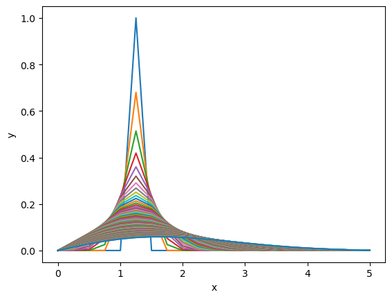
Let us try with an initial peak somewhere in the middle.

Lx = 5   # length
N = 20   # division in space
x = np.linspace(0, Lx, N+1)  # positions
y0 = np.zeros_like(x)  # initial condition
y0[5] = 1   # 1 at left end

D = 0.1  # diffusion constant
dt = 0.1 # time step
ts = 10.   # time for solution
y = euler(diff1D, y0, dt, int(ts/dt), (x, D))
# spatial pattern at different time
plt.plot(x, y.T)
plt.xlabel("x"); plt.ylabel("y");

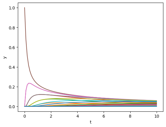
# evolution of each point in time
t = np.arange(0,ts+dt,dt)
plt.plot(t,y)
plt.xlabel("t"); plt.ylabel("y");

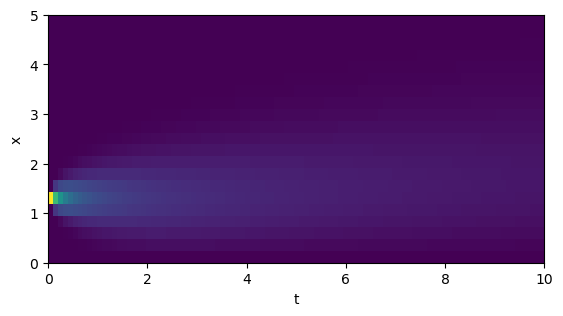
# plot in space and time
plt.imshow(y.T, origin='lower', extent=(0, ts, 0, Lx))
plt.xlabel("t"); plt.ylabel("x");

The accuracy of solution depends on the fineness of discretization in space and time.

Let us try a finer spatial division.

N = 40  # discretization in space
x = np.linspace(0, Lx, N+1)
y0 = np.zeros_like(x)  # initial condition
y0[10] = 1   # initial peak at x=10/50
y = euler(diff1D, y0, dt, int(ts/dt), (x, D))
# evolution of spatial pattern
plt.plot(x, y.T)
plt.xlabel("x"); plt.ylabel("y");

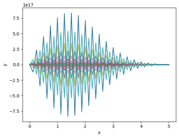
In the diffusion equation, peaks are pulled down and dips are pushed up, and that can cause spatial instability if the time step is too large.

# plot in space and time
plt.imshow(y[:10].T, origin='lower', extent=(0, ts, 0, Lx))
plt.xlabel("t"); plt.ylabel("x");

Stability

For an accurate solution, \(\Delta x\) have to be small. But making \(\Delta x\) small can make the ODE stiff such that solution can be unstable.
It is known that stable solution by Euler method requires

\[ \Delta t \le \frac{\Delta x^2}{2D}. \]

In the above example, \(\Delta t=0.1\) was over the limit:

(Lx/N)**2/(2*D)

0.078125

By odeint

The above stability issue can be worked around by using an ODE library that implements automatic time step adaptation, such as odeint.

from scipy.integrate import odeint

Lx = 5   # length
N = 40
x = np.linspace(0, Lx, N+1)
y0 = np.zeros_like(x)  # initial condition
y0[10] = 1
D = 0.1  # diffusion constant
dt = 0.1
ts = 10
t = np.arange(0, ts, dt)
y = odeint(diff1D, y0, t, (x, D))
# evolution of spatial pattern
p = plt.plot(x, y.T)
plt.xlabel("x"); plt.ylabel("y");

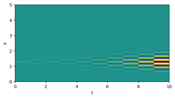
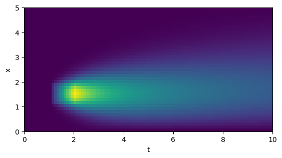
Let us see the case with an input.

def pulse(y, x, t):
    """1 for 1<x<2 at 1<t<2"""
    return (1<x)*(x<2)*(1<t)*(t<2)*1.

N = 40
x = np.linspace(0, Lx, N+1)
y0 = np.zeros_like(x)  # initial condition
t = np.arange(0, ts, dt)
y = odeint(diff1D, y0, t, (x, D, pulse))
# plot in space and time
plt.imshow(y.T, origin='lower', extent=(0, ts, 0, Lx))
plt.xlabel("t"); plt.ylabel("x");

3D plot and animation

For more intuitive visualization of the space-time dynamics, you may want to use 3D plot or animation.

# uncomment the line below for interactive graphics
#%matplotlib notebook

# plot in 3D
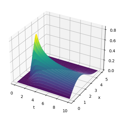
fig = plt.figure()
ax = fig.add_subplot(projection='3d')
T, X = np.meshgrid(t, x)
ax.plot_surface(T, X, y[:,:N+1].T, cmap='viridis')
plt.xlabel("t"); plt.ylabel("x"); 

from matplotlib import animation

fig = plt.figure()
frames = []  # prepare frame
for i, ti in enumerate(t):
    p = plt.plot(x, y[i], 'b')
    plt.xlabel("x"); plt.ylabel("y");
    frames.append(p)    
anim = animation.ArtistAnimation(fig, frames, interval = 10)

%matplotlib inline

Boundary Conditions

As briefly mentioned above, there are two typical ways of specifying the boundary condition:

• Dirichlet boundary condition: the value \(y(x_0,t)=y_0\) or \(y(x_N,t)=y_N\)

  • concentration at an open end of a tube to a water bath.

  • voltage of an electric cable attached to the ground or a strong battery.

• Neumann boundary condition: the derivative \(\left.\frac{\partial y(x,t)}{\partial x}\right|_{x_0}=y'_0\) or \(\left.\frac{\partial y(x,t)}{\partial x}\right|_{x_N}=y'_N\)

  • concentration at a closed end of a tube (no molecular flow).

  • voltage at a dead end of an electric cable.

We already implemented Dirichlet boundary condition in diff1D().

Let us implement a Neumann boundary condition at the right end \(\left.\frac{\partial y(x,t)}{\partial x}\right|_{x_N}=0\) and see the difference.

A simple way is to use a one-sided differentiation

\[ \frac{\partial y}{\partial x} \simeq \frac{y_{N+1}-y_{N}}{\Delta x}=0\]

which reduces to \(y_{N+1}=y_{N}\) and

\[ \frac{dy_N}{dt} = D \frac{y_{N-1} - 2y_N + y_{N+1}}{\Delta x^2} = D \frac{y_{N-1} - y_N}{\Delta x^2}.\]

A better way is to use a symmetric differentiation

\[ \frac{\partial y}{\partial x} \simeq \frac{y_{N+1}-y_{N-1}}{2\Delta x}=0\]

which reduces to \(y_{N+1}=y_{N-1}\) and

\[ \frac{dy_N}{dt} = D \frac{y_{N-1} - 2y_N + y_{N+1}}{\Delta x^2} = 2D \frac{y_{N-1} - y_N}{\Delta x^2}.\]

def diff1DN(y, t, x, D, inp=None):
    """1D Diffusion equaiton with boundary conditions
    y_0=0 on the left and dy/dx|x_N=0 on the right end.
    y: state vector
    t: time
    x: positions
    D: diffusion coefficient
    input: function(y,x,t)"""
    # spatial step
    dx = x[1] - x[0]
    # shift array to left and right
    d2ydx2 = (y[:-2] -2*y[1:-1] + y[2:])/dx**2
    # Dirichlet on the left, Neumann on the right end
    d2ydx2 = np.hstack((0, d2ydx2, 2*(y[-2] - y[-1])/dx**2))
    if inp == None:
        return(D*d2ydx2)
    else:
        return(D*d2ydx2 + inp(y, x, t))

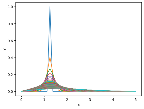
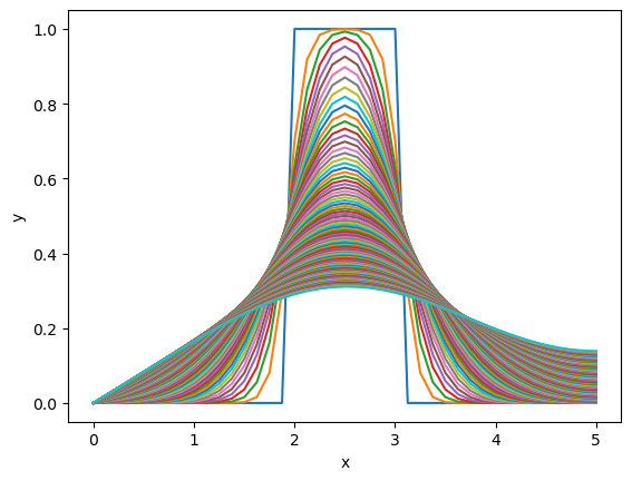
For example, from the initial bump in the center, the spreads to both sides are quite different.

N = 40
x = np.linspace(0, Lx, N+1)
y0 = np.zeros_like(x)  # initial condition
y0[16:25] = 1
ts = 10
t = np.arange(0, ts, dt)
y = odeint(diff1DN, y0, t, (x, D))
# evolution of spatial pattern
plt.plot(x, y.T)
plt.xlabel("x"); plt.ylabel("y");

Wave Equation

PDE with a second-order dynamics can represent traveling waves. The wave equation has the standard form

\[ \frac{\partial^2 u}{\partial t^2} + d\frac{\partial u}{\partial t} = c^2 \frac{\partial^2 u}{\partial x^2}\]

where \(c\) is the wave speed and \(d\) is the decay rate.

We convert the second-order system to a set of first order systems by consiering a vector \(y=(u,v)\) representing the amplitude \(u\) and its change rate \(v\):

\[ \frac{\partial u}{\partial t} = v \]

\[ \frac{\partial v}{\partial t} = c^2 \frac{\partial^2 u}{\partial x^2} - dv \]

def wave1D(y, t, x, c, d, inp=None):
    """1D wave equaiton with constant boundary
    y: state vector hstack(u, v)
    t: time
    x: positions
    c: wave speed
    input: function(y,x,t)"""
    n = int(len(y)/2)
    u, v = y[:n], y[n:]
    dx = x[1] - x[0]
    # finite different approximation
    d2udx2 = (u[:-2] -2*u[1:-1] + u[2:])/dx**2
    d2udx2 = np.hstack((0, d2udx2, 0))  # add 0 to both ends
    if inp == None:
        return np.hstack((v, c**2*d2udx2 - d*v))
    else:
        return np.hstack((v, c**2*d2udx2 - d*v + inp(y, x, t)))

Lx = 10
N = 100
x = np.linspace(0, Lx, N+1)
c = 1.  # wave speed
d = 0.1
ts = 30
dt = 0.1
t = np.arange(0, ts, dt)
y0 = np.zeros(2*(N+1))  # initial condition
#y0[20:40] = 1
#y = odeint(wave1D, y0, t, (x, c, d))
y = odeint(wave1D, y0, t, (x, c, d, pulse))
# plot in space and time
# show only first dimension
plt.imshow(y[:,:N+1].T, origin='lower', extent=(0, ts, 0, Lx))
plt.xlabel("t"); plt.ylabel("x");

#evolution in spatial pattern
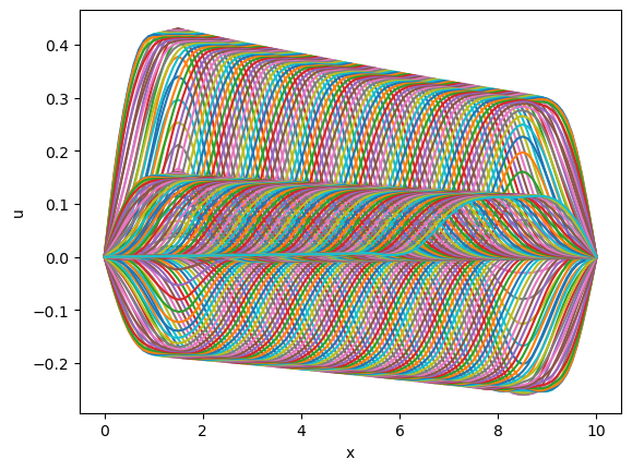
plt.plot(x, y[:,:N+1].T)  # only first dimension
plt.xlabel("x"); plt.ylabel("u"); 

# plot in 3D
fig = plt.figure(figsize=(8, 8))
ax = fig.add_subplot(projection='3d')
T, X = np.meshgrid(t, x)
ax.plot_surface(T, X, y[:,:N+1].T, cmap='viridis')
plt.xlabel("t"); plt.ylabel("x"); 

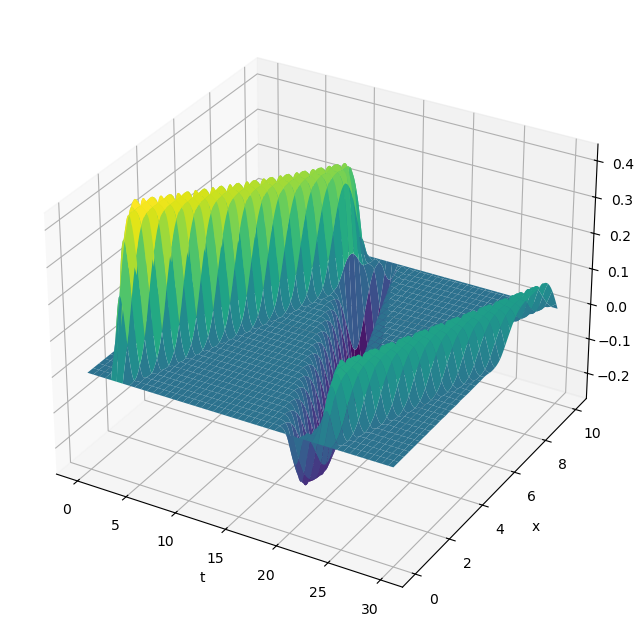
fig = plt.figure()
frames = []  # prepare frame
for i, ti in enumerate(t):
    p = plt.plot(x, y[i,:N+1])
    plt.xlabel("x"); plt.ylabel("y");
    frames.append(p)    
anim = animation.ArtistAnimation(fig, frames, interval = 10)

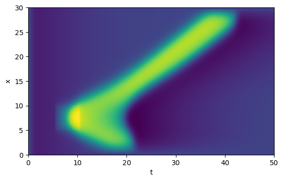
Reaction-Diffusion Equation

Linear waves can decay, reflect, and overlay.
Some nonlinear waves, like neural spike, can travel without decaying. FitzHugh-Nagumo model can be embedded in a diffusive axon model

\[ \frac{\partial v}{\partial t} = v - \frac{v^3}{3} - w + D\frac{\partial^2 v}{\partial x^2} + I \]

\[ \frac{\partial w}{\partial t} = \phi (v + a - bw) \]

def fhnaxon(y, t, x, inp=0, D=1, a=0.7, b=0.8, phi=0.08):
    """FitzHugh-Nagumo axon model
    y: state vector hstack(v, w)
    t: time
    x: positions
    I: input current
    D: diffusion coefficient
    """
    n = int(len(y)/2)
    v, w = y[:n], y[n:]
    # finite difference approximation
    d2vdx2 = (v[:-2] -2*v[1:-1] + v[2:])/(x[1] - x[0])**2
    d2vdx2 = np.hstack((0, d2vdx2, 0))  # add 0 to both ends
    I = inp(y,x,t) if callable(inp) else inp # function or constant
    dvdt = v - v**3/3 - w + D*d2vdx2 + I
    dwdt = phi*(v + a -b*w)
    return(np.hstack((dvdt, dwdt)))

def pulse2(y, x, t):
    """1 for 5<x<10 at 5<t<10"""
    return (5<x)*(x<10)*(5<t)*(t<10)

Lx = 30
N = 100
x = np.linspace(0, Lx, N+1)
y0 = np.zeros(2*(N+1))  # initial condition
y0[0:N+1] = -1.2  # initialize near the resting state
ts = 50
dt = 0.5
t = np.arange(0, ts, dt)
y = odeint(fhnaxon, y0, t, (x, pulse2))
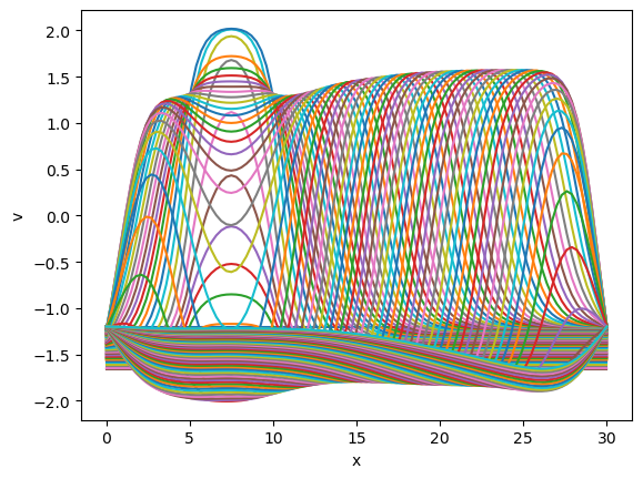
# evolution of spatial pattern in time
p = plt.plot(x, y[:,:N+1].T) # plot in space
plt.xlabel("x"); plt.ylabel("v");

# in space and time
plt.imshow(y[:,:N+1].T, origin='lower', extent=(0, ts, 0, Lx))
plt.xlabel("t"); plt.ylabel("x");

#%matplotlib notebook

# plot in 3D
fig = plt.figure()
ax = fig.add_subplot(projection='3d')
T, X = np.meshgrid(t, x)
ax.plot_surface(T, X, y[:,:N+1].T, cmap='viridis')
plt.xlabel("t"); plt.ylabel("x"); 

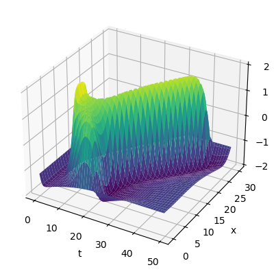
fig = plt.figure()
frames = []  # prepare frame
for i, ti in enumerate(t):
    p = plt.plot(x, y[i,:N+1])
    plt.xlabel("x"); plt.ylabel("y");
    frames.append(p)    
anim = animation.ArtistAnimation(fig, frames, interval = 10)

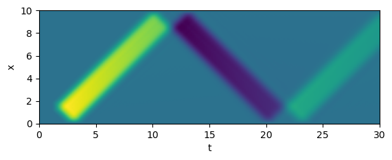
Cyclic Boundary Condition

A practical way to approximate an infinitely large space without the effect of boundaries is to use the cyclic or periodic boundary condition, in which both ends of the space is assumed to be connected, like a ring, torus, etc.

You can use np.roll function to shift the contents of an array as a ring.

def fhnaxon_cb(y, t, x, inp=0, D=1, a=0.7, b=0.8, phi=0.08):
    """FitzHugh-Nagumo axon model
    y: state vector hstack(v, w)
    t: time
    x: positions
    I: input current
    D: diffusion coefficient
    """
    n = int(len(y)/2)
    v, w = y[:n], y[n:]
    # cyclic boundary condition
    d2vdx2 = (np.roll(v,-1) -2*v + np.roll(v,1))/(x[1] - x[0])**2
    # If inp is a function, call it with arguments. Otherwise take it as a constant
    I = inp(y,x,t) if callable(inp) else inp
    dvdt = v - v**3/3 - w + D*d2vdx2 + I
    dwdt = phi*(v + a -b*w)
    return(np.hstack((dvdt, dwdt)))

y = odeint(fhnaxon_cb, y0, t, (x, pulse2))
# in space and time
plt.imshow(y[:,:N+1].T, origin='lower', extent=(0, ts, 0, Lx))
plt.xlabel("t"); plt.ylabel("x");

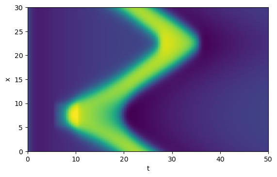
In this example, the propagate in both directions and the one left at the bottom reappears from the top. Then the two spikes collide and disappear.

PDE in 2D space

We can also model dynamics in two or higher dimension spate.

The diffusion equation of a variable \(y(x_1,x_2,t)\) in the 2D space is given by:

\[\frac{\partial y}{\partial t} = D\frac{\partial^2 y}{\partial x_1^2} + D\frac{\partial^2 y}{\partial x_2^2} + g(y, x, t)\]

Using the Laplace operator (or Laplacian):

\[\nabla^2 = \frac{\partial^2}{\partial x_1^2} + \frac{\partial^2}{\partial x_2^2}\]

the diffusion equation is represented as

\[\frac{\partial y}{\partial t} = D\nabla^2 y + g(y, x, t)\]

Diffusion equation in 2D space

Like the case in 1D space, we discretize the space in a 2D grid, and covert the PDF to ODE.

def diff2D(y, t, x, D, inp=0):
    """1D Diffusion equaiton with constant boundary condition
    y: states at (x0, x1)
    t: time
    x: positions (x0, x1) in meshgrid format
    D: diffusion coefficient
    inp: function(y,x,t) or number"""
    n = np.array(x).shape[1:]  # grid size (n0, n1)
    nn = n[0]*n[1]  # grid points n0*n1
    y = y.reshape(n)  # linear to 2D
    dx = [x[0,0,1]-x[0,0,0], x[1,1,0]-x[1,0,0]]  # space step
    # Laplacian with cyclic boundary condition
    Ly = (np.roll(y,-1,0)+np.roll(y,1,0)-2*y)/dx[0]**2 + (np.roll(y,-1,1)+np.roll(y,1,1)-2*y)/dx[1]**2
    # fix the boundaris to 0 for Dirichlet condition
    Ly[0,:] = Ly[-1,:] = Ly[:,0] = Ly[:,-1] = 0
    dydt = D*Ly + (inp(y,x,t) if callable(inp) else inp)
    return dydt.ravel()

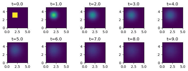
L = 5
N = 20
x = np.array(np.meshgrid(np.linspace(0,L,N), np.linspace(0,L,N)))
ts = 10
dt = 0.1
t = np.arange(0, ts, dt)
D = 0.1
y0 = np.zeros((N,N))  # initial condition
y0[5:10,10:15] = 1  # initial bump
y = odeint(diff2D, y0.ravel(), t, (x, D))

plt.figure(figsize=(8,3))
for i in range(10):
    plt.subplot(2, 5, i+1)
    plt.imshow(y[10*i].reshape(N,N).T, vmin=0, vmax=1, origin='lower', extent=(0,L,0,L))
    plt.title('t={:1.1f}'.format(t[10*i]))
plt.tight_layout()

# animation
fig = plt.figure()
frames = []  # prepare frame
for i, ti in enumerate(t):
    p = plt.imshow(y[i].reshape(N,N).T, vmin=0, vmax=1, origin='lower', extent=(0,L,0,L))
    frames.append([p])    
anim = animation.ArtistAnimation(fig, frames, interval = 10)
plt.xlabel("x1"); plt.ylabel("x2");

PDE libraries

Solution of PDE is computationally intensive, especially in 2D or higher dimensional space. For practical computation, it is better to use specialized libraries for solving PDEs, such as:

• py-pde: https://py-pde.readthedocs.io

• FiPy: https://www.ctcms.nist.gov/fipy

• FEniCS: https://fenicsproject.org