6. Ordinary Differential Equations

\[ % Latex macros \newcommand{\mat}[1]{\begin{pmatrix} #1 \end{pmatrix}} \newcommand{\p}[2]{\frac{\partial #1}{\partial #2}} \newcommand{\b}[1]{\boldsymbol{#1}} \newcommand{\w}{\boldsymbol{w}} \newcommand{\x}{\boldsymbol{x}} \newcommand{\y}{\boldsymbol{y}} \]

A differential equation is an equation that includes a derivative \(\frac{df(x)}{dx}\) of an unknown function \(f(x)\).

The derivative means the slope, mathematically defined as the limit:

\[ \frac{df(x)}{dx} = \lim_{\Delta x \rightarrow 0} \frac{f(x+\Delta x) - f(x)}{\Delta x} \]

A differential equation including a derivative by only one variable is called an ordinary differential equation (ODE).

Here we consider ODEs of the form

\[ \frac{dy}{dt} = f(y, t) \]

which describes the temporal dynamics of a varibale \(y\) over time \(t\). It is also called a continuous-time dynamical system.

Finding the variable as an explicit function of time \(y(t)\) is called solving or integrating the ODE. When it is done numerically, it is aslo called simulating.

References:

• Strogatz SH (2024). Nonlinear Dynamics And Chaos.

• Scientific Python Lectures: Section 1.5.7 Numerical Integration

Basics of derivatives

Here are some basic properties of the derivative \(f'(x)=\frac{df(x)}{dx}\)

• The derivative of a polynomial:

\[ (x^n)' = n x^{n-1} \]

• The derivative of exponential is itself:

\[ (e^x)' = e^x \]

• Derivatives of sine and cosine:

\[ \sin'(x)=\cos(x),\]

\[ \cos'(x)=-\sin(x) \]

• Linearity:

\[ (af(x)+bg(x))' = af'(x)+bg'(x) \]

• Chain rule:

\[ (f(g(x))' = f'(g(x))g'(x) \]

Second-order derivative

The second-order derivative \(\frac{d^2f(x)}{dx^2}\) of a function \(f(x)\) is the derivative of the derivative:

\[ \frac{d^2f(x)}{dx^2} = \frac{d}{dx}\frac{df(x)}{dx} = \lim_{\Delta x \rightarrow 0} \frac{f(x+\Delta x) - 2f(x) + f(x-\Delta x)}{\Delta x^2} \]

A second-order derivative represents the change in the slope, i.e., the curvature.

Analytic Solutions

Solving a differential equation is an inverse problem of differentiation, for which analytic solution may not be available.

The simplest case where analytic solutions are available is linear differential equations

\[ \frac{dy}{dt} = A y \]

where \(y\) is a real variable or a real vector, and \(A\) is a constant coefficient or a matrix.

Linear ODEs

In general, a differential equation can have multiple solutions. For example, for a scalar linear ODE

\[ \frac{dy(t)}{dt} = a y(t), \]

a solution is given by

\[ y(t) = e^{at}. \]

Finding a solution of an ODE is generally not easy, but verifying a solution is relatively easy. In the above case, you can verify it by the chain rule as :

\[ \frac{dy(t)}{dt} = \frac{de^{at}}{dt} = \left.\frac{de^{x}}{dx}\right|_{x=at}\frac{dat}{dt} = e^{at}a = a y(t). \]

However, this is not the only solution. In fact, all scaled variants

\[ y(t) = C e^{at}, \]

where \(C\) can be any real value, are solutions.

• Verify that by differentiating both sides of the equaiton above.

When the value of \(y(t)\) at a certain time \(t\) is specified, the solution becomes unique.
For example, by specifying an initial condition

\[ y(0)=3, \]

from \(e^{a0}=e^0=1\), we have \(C=3\) and a particular solution $\( y(t)=3e^{at} \)$ is determined.

Finding a solution from a given initial value \(y(0)\) is called an initial value problem.

For a second-order linear ODE

\[ \frac{d^2y}{dt^2} = -a^2 y, \]

the solution is given by

\[ y(t) = C_1 \sin at + C_2 \cos at \]

where \(C_1\) and \(C_2\) are determined by specifying \(y\) and \(dy/dt\) at certain time.

• Also verify this by differentiation.

Analytically solvable ODEs

Other cases where analytic solutions are well known are:

• Linear time-varying coefficient:

\[ \frac{dy}{dt} = a(t)y \]

\(at\) replaced by time integral \(\int a(t)dt\)

\[ y(t) = C e^{\int a(t)dt} \]

• Linear time-varying input:

\[\frac{dy}{dt} = a(t)y + b(t)\]

using the above solution \(y_0(t)\) for \(b(t)=0\)

\[ y(t) = Cy_0(t) + y_0(t) \int \frac{b(t)}{y_0(t)}dt \]

• Separation of variables:

\[\frac{dy}{dt} = a(y)b(t)\]

two related integrals

\[\int \frac{1}{a(y)}dy = \int b(t)dt + C \]

• Other cases that can be reduced to above by change of variables, etc.

You can use dsolve() function of SymPy to find some analitic solutions. See Scipy Tutorial, Chapter 16 if you are interested.

Euler Method

The most basic way of solving an ODE numerically is Euler Method.
For an ODE

\[ \frac{dy}{dt} = f(y,t), \]

we approximate the derivative with the finite difference

\[ \frac{dy}{dt} \simeq \frac{y(t+\Delta t) - y(t)}{\Delta t} = f(y,t) \]

and reorder this to predict \( y(t+\Delta t) \) as

\[ y(t+\Delta t) = y(t) + f(y,t) \Delta t. \]

We can use this iteratively from an initial value \(y(0)\) with a small time step \(\Delta t\) to approximate the solution.

import numpy as np
import matplotlib.pyplot as plt
%matplotlib inline

def euler(f, y0, dt, n, *args):
    """f: righthand side of ODE dy/dt=f(y,t)
        y0: initial condition y(0)=y0
        dt: time step
        n: iteratons
        args: parameter for f(y,t,*args)"""
    d = np.array([y0]).size  ## state dimension
    y = np.zeros((n+1, d))
    y[0] = y0
    t = 0
    for k in range(n):
        y[k+1] = y[k] + f(y[k], t, *args)*dt
        t = t + dt
    return y

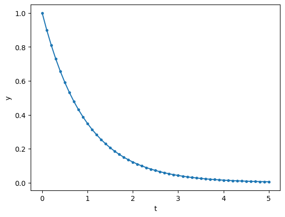
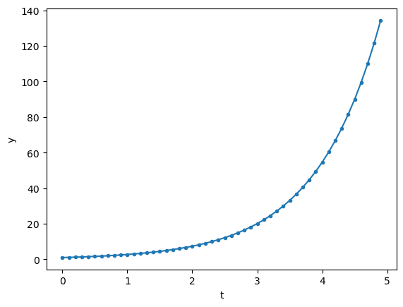
Let us test this with a first-order linear ODE.

def first(y, t, a):
    """first-order linear ODE dy/dt = a*y"""
    return a*y

dt = 0.1 # time step
T = 5    # time span
n = int(T/dt)  # steps
t = np.linspace(0, T, n+1)
y = euler(first, 1, dt, n, -1)
plt.plot(t, y, '.-')
plt.xlabel('t'); plt.ylabel('y');

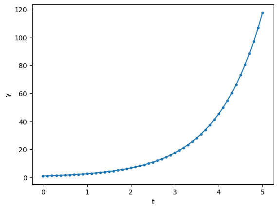
y = euler(first, 1, dt, n, 1)
plt.plot(t, y, '.-')
plt.xlabel('t'); plt.ylabel('y');

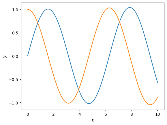
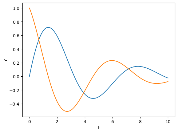
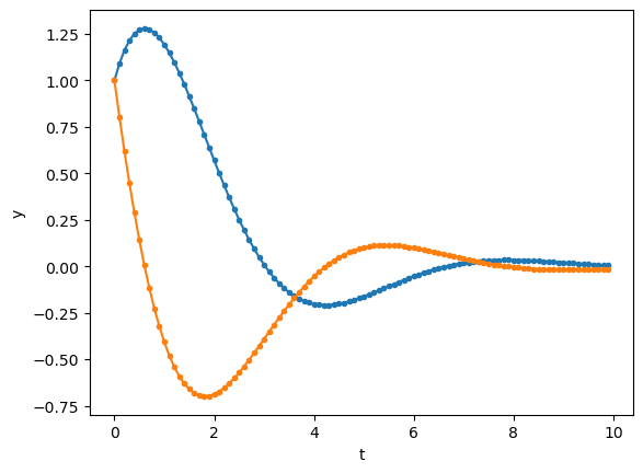
A second-order ODE

\[ \frac{d^2y}{dt^2} = a_2 \frac{dy}{dt} + a_1 y + a_0 \]

can be converted into a first-order ODE of a 2-dimensional vector \({\bf y} = \pmatrix{y_1 \\ y_2} =\pmatrix{y \\ \frac{dy}{dt}}\) as

\[ \frac{dy_1}{dt} = y_2 \]

\[ \frac{dy_2}{dt} = a_2 y_2 + a_1 y_1 + a_0 \]

or in a vector-matrix form

\[ \frac{d}{dt}{\bf y} = A{\bf y} + {\bf b}\]

where

\[\begin{split} A = \pmatrix{0 & 1 \\ a_1 & a_2} \mbox{ and } {\bf b} = \pmatrix{0 \\ a_0}\end{split}\]

def second(y, t, a):
    """second-order linear ODE """
    y1, y2 = y
    return np.array([y2, a[2]*y2 + a[1]*y1 + a[0]])

dt = 0.01 # time step
T = 10    # time span
n = int(T/dt)  # steps
t = np.linspace(0, T, n+1)
y = euler(second, [0, 1], dt, n, [0, -1, 0])
plt.plot(t, y);
plt.xlabel('t'); plt.ylabel('y');

y = euler(second, [0, 1], dt, n, [0, -1, -0.5])
plt.plot(t, y)
plt.xlabel('t'); plt.ylabel('y');

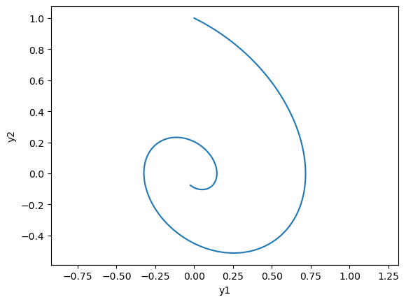
# phase plot
plt.plot(y[:,0], y[:,1]);
plt.xlabel('y1'); plt.ylabel('y2'); plt.axis('equal');

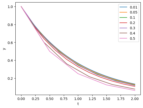
Let us see how the time step affects the accuracy of the solution.

steps = [0.01, 0.05, 0.1, 0.2, 0.3, 0.4, 0.5]
T = 2
a = -1
for dt in steps:
    n = int(T/dt)  # steps
    t = np.linspace(0, T, n+1)
    y = euler(first, 1, dt, n, a)
    plt.plot(t,y)
plt.xlabel('t'); plt.ylabel('y'); plt.legend(steps);

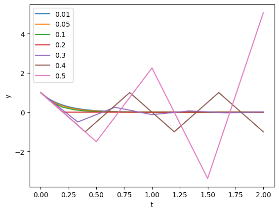
a = -5
for dt in steps:
    n = int(T/dt)  # steps
    t = np.linspace(0, T, n+1)
    y = euler(first, 1, dt, n, a)
    plt.plot(t,y)
plt.xlabel('t'); plt.ylabel('y'); plt.legend(steps);

Scipy’s Integrate package

To avoid numerical instability and to improve accuracy and efficiency, there are advanced methods for ODE solutions.

• Backward Euler method: solve

\[ y(t+\Delta t) = y(t) + f(y(t+\Delta t)) \Delta t\]

• Mixture of forward and backward (Crank-Nicolson):

\[ y(t+\Delta t) = y(t) + \frac{1}{2}\{f(y(t))+f(y(t+\Delta t))\} \Delta t\]

• Runge-Kutta method: minimize higher-order erros by Taylor expansion

\[ y(t+\Delta t) = y(t) + f(y(t))\Delta t + \frac{1}{2} \frac{d}{dt}f(y(t))\Delta t^2 + ...\]

• Adative time step: adjust \(\Delta t\) depending on the scale of \(\frac{df(y(t))}{dt}\).

The implementation and choice of these methods require a good expertise, but fortunately scipy includes integrate package which has been well tested and optimized.
odeint() implements automatic method switching and time step adaptation.
Alternatively, you can use a new function solve_ivp(), with a different function definition as f(t, y).

from scipy.integrate import odeint

#help(odeint)

Here is an example of first-order linear ODE.

t = np.arange(0, 5, 0.1)  # time points
y = odeint(first, 1, t, args=(1,))
plt.plot(t, y, '.-');
plt.xlabel('t'); plt.ylabel('y');

Here’s another example of second-order linear ODE.

t = np.arange(0, 10, 0.1)  # time points
y = odeint(second, [1, 1], t, args=([0, -1, -1],))
plt.plot(t, y, '.-');
plt.xlabel('t'); plt.ylabel('y');

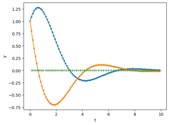
odeint() internally uses adaptive time steps, and returns values of y for time points specified in t by interpolation.

# If you are interested in the internal time steps used...
t = np.arange(0, 10, 0.1)  # time points
y, info = odeint(second, [1, 1], t, args=([0, -1, -1],), full_output=1)
#y, info = odeint(first, 1, t, args=(-1,), full_output=1)
plt.plot(t, y, '.-')
# the crosses show the time points actually used
plt.plot(info['tcur'], np.zeros_like(info['tcur']), '+');
plt.xlabel('t'); plt.ylabel('y');

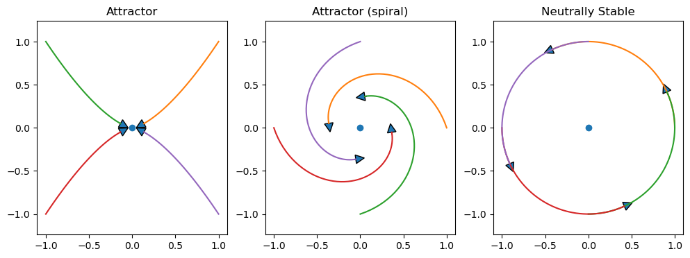
Fixed Point and Stability

A point \(y\) that satisfy \(\frac{d}{dt}{\bf y}=f({\bf y})={\bf 0}\) is called a fixed point.

A fixed point is characterized by its stability.

def expos(a, b):
    """Exponentials exp(a*t), exp(b*t)"""
    u = np.array(np.exp(a*t))
    v = np.array(np.exp(b*t))
    x = np.array([u, -u, -u, u]).T
    y = np.array([v, v, -v, -v]).T
    return x, y

def spirals(a, b):
    """Spirals: exp(a*t)*cos(b*t), exp(a*t)*sin(b*t) """
    u = np.array(np.exp(a*t)*np.cos(b*t))
    v = np.array(np.exp(a*t)*np.sin(b*t))
    x = np.array([u, v, -u, -v]).T
    y = np.array([v, -u, -v, u]).T
    return x, y

def arrowcurves(x, y, s=0.1):
    """curves with an arrowhead
    x, y: time courses in columns
    s: arrowhead size"""
    plt.plot(x, y)
    n = x.shape[1]  # columns
    for i in range(n):
        plt.arrow(x[-2,i], y[-2,i], x[-1,i]-x[-2,i], y[-1,i]-y[-2,i],
                 head_width=s, head_length=s)
    plt.axis('equal')
    

t = np.linspace(0, 1)  # time points

• Stable

  • Attractor

  • Neutrally stable

plt.figure(figsize=(12,4))
plt.subplot(1,3,1)
plt.title('Attractor')
plt.plot(0, 0, 'o')
x, y = expos(-2, -3)
arrowcurves(x, y)
plt.subplot(1,3,2)
plt.title('Attractor (spiral)')
plt.plot(0, 0, 'o')
x, y = spirals(-1, 3)
arrowcurves(x,y)
plt.subplot(1,3,3)
plt.title('Neutrally Stable')
plt.plot(0, 0, 'o')
x, y = spirals(0, 2)
arrowcurves(x,y)

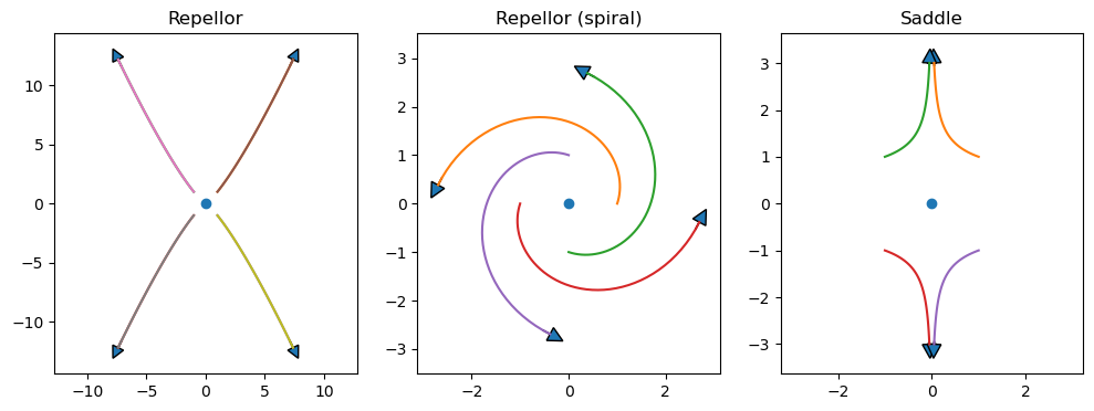
• Unstable

  • repellor

  • Saddle

plt.figure(figsize=(12,4))
plt.subplot(1,3,1)
plt.title('Repellor')
plt.plot(0, 0, 'o')
x, y = expos(2, 2.5)
arrowcurves(x, y, s=1)
arrowcurves(x, y)
plt.subplot(1,3,2)
plt.title('Repellor (spiral)')
plt.plot(0, 0, 'o')
x, y = spirals(1, 3)
arrowcurves(x, y, s=0.3)
plt.subplot(1,3,3)
plt.title('Saddle')
plt.plot(0, 0, 'o')
x, y = expos(-3, 1.1)
arrowcurves(x, y, s=0.3)

Linear dynamical system

For a linear dynamical system

\[ \frac{d}{dt}{\bf y} = A {\bf y} \]

where \({\bf y}\) is an \(n\) dimensional vector and \(A\) is an \(n\times n\) matrix, the origin \({\bf y}={\bf 0}\) is always a fixed point. Its stability is determined by the eigenvalues of \(A\).

• If the real part of all the eigenvalues are negative or zero, the system is stable.

• If any of the real part of the eigenvalues is positive, the system is unstable.

• If there are complex eigenvalues, the solution is oscillatory.

def linear(y, t, A):
    """Linear dynamcal system dy/dt = Ay
    y: n-dimensional state vector
    t: time (not used, for compatibility with odeint())
    A: n*n matrix"""
    # y is an array (row vector), A is a matrix
    return A@y

def lode_plot(A, y0=[1,0]):
    """Plot the trajectory and eiven values of linear ode"""
    ev,_ = np.linalg.eig(A)
    print('A =', A, '\nev =', ev)
    t=np.arange(0, 10, 0.1)
    y = odeint(linear, y0, t, args=(A,))
    plt.plot(y[0,0], y[0,1], 'o')   # starting point
    plt.plot(y[:,0], y[:,1], '.-')  # trajectory
    plt.plot(y[-1,0], y[-1,1], '*')  # end point
    plt.axis('equal')

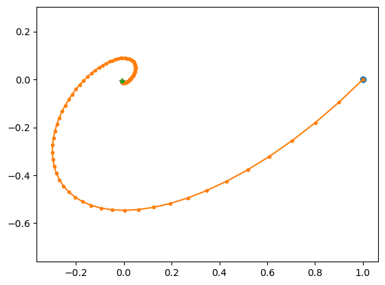
Try different settings of A.

# spiral in
lode_plot([[-1, 1], [-1, 0]])

A = [[-1, 1], [-1, 0]] 
ev = [-0.5+0.8660254j -0.5-0.8660254j]

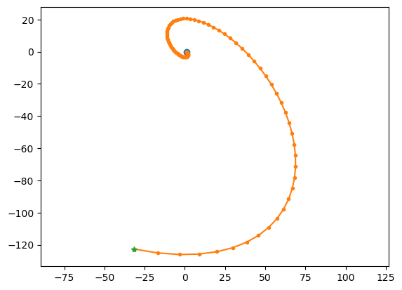
# spiral out
lode_plot([[1, 1], [-1, 0]])

A = [[1, 1], [-1, 0]] 
ev = [0.5+0.8660254j 0.5-0.8660254j]

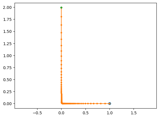
# saddle point
lode_plot([[-1, 0], [0, 1]], [1,0.0001])

A = [[-1, 0], [0, 1]] 
ev = [-1.  1.]

Nonlinear ODEs

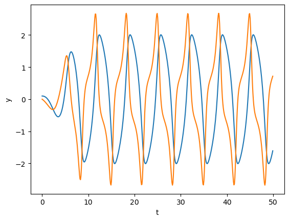
While the dynamics of a linear ODE can show only convergence, divergence, or neutrally stable oscillations, nonlinear ODEs can show limit-cycle oscillation and chaos.

Van der Pol oscillator

This is a classic equation describing an oscillator circuit with a vacuume tube:

\[ \frac{d^2y}{dt^2} - \mu(1-y^2)\frac{dy}{dt} + y = 0 \]

This can be converted into a 2D system as

\[ \frac{dy_1}{dt} = y_2 \]

\[ \frac{dy_2}{dt} = \mu(1-y_1^2)y_2 - y_1 \]

def vdp(y, t, mu=1.):
    """Van der Pol equation"""
    y1, y2 = y
    return np.array([y2, mu*(1 - y1**2)*y2 - y1])

t = np.arange(0, 50, 0.1)
y = odeint(vdp, [0.1, 0], t)
plt.plot(t, y);
plt.xlabel('t'); plt.ylabel('y');

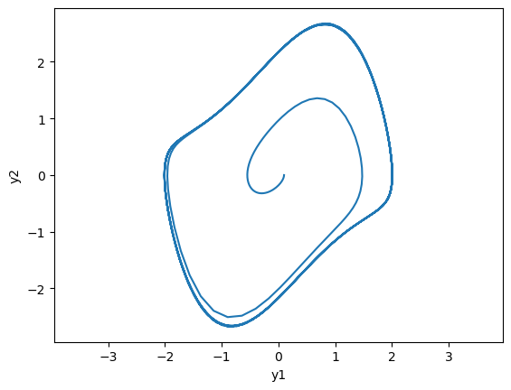
# phase plot
plt.plot(y[:,0], y[:,1]);
plt.xlabel('y1'); plt.ylabel('y2'); plt.axis('equal');

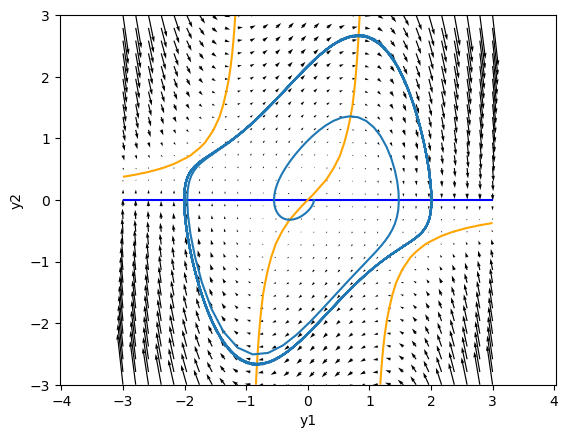
Nullclines

The dynamincs in a 2D space is well characterized by the nullclines, the lines where \(\frac{dy_i}{dt}=0\).

For the Van del Pol oscillator, they are given by:

\[ \frac{dy_1}{dt} = 0 \rightarrow y_2 = 0 \]

\[ \frac{dy_2}{dt} = 0 \rightarrow y_2 = \frac{y_1}{\mu(1-y_1^2)} \]

Above the \(\frac{dy_1}{dt} = 0\) nullcline, \(\frac{dy_1}{dt} > 0\), so the points move toward the right, and below the nullcline, points move toward left.
On the right side of the \(\frac{dy_2}{dt} = 0\) nullcline in the center, \(\frac{dy_2}{dt} > 0\), so the points move downward, and on the left side, points move upward.

The crosspoint of the two nullclines is a fixed point \(\frac{dy_1}{dt} = \frac{dy_2}{dt} = 0\).

m = 30
x = np.linspace(-3, 3, m)
X, Y = np.meshgrid(x, x)
mu = 1
Z = vdp([X, Y], 1, mu)
plt.contour(X, Y, Z[0], levels=[0], colors='blue')  # dy1/dt = 0
plt.contour(X, Y, Z[1], levels=[0], colors='orange')  #dy2/dt = 0
plt.quiver(X, Y, Z[0], Z[1])   # vector field
y = odeint(vdp, [0.1, 0], t, args=(mu,))  # solve ODE
plt.plot(y[:,0], y[:,1]);  # solution
plt.xlabel('y1'); plt.ylabel('y2'); plt.axis('equal');

The stability of the fixed point is determined by the eigenvalues of the linearized system

\[ \frac{d\b{x}}{dt} = A \b{x} \]

where \(A = \p{\b{f}(\b{y})}{\b{y}}\) is the Jacobian matrix at the fixed point.

For the Van der Pol oscillator, the Jacobian at the fixed point \(\b{y}=(0,0)^T\) is:

\[\begin{split} A = \mat{0 & 1 \\ -2\mu y_1 - 1 & \mu(1-y_1^2)} = \mat{0 & 1 \\ -1 & \mu} \end{split}\]

Its eigenvalues are \(\mu/2 + \sqrt{\mu^2/4-1}\), which is complex with positive real part for \(\mu<2\), makeing the trajectory near the fixed point spiraling out.

A = np.array([[0, 1], [-1, mu]])
np.linalg.eig(A)

EigResult(eigenvalues=array([0.5+0.8660254j, 0.5-0.8660254j]), eigenvectors=array([[0.70710678+0.j        , 0.70710678-0.j        ],
       [0.35355339+0.61237244j, 0.35355339-0.61237244j]]))

Please try with different values of \(\mu\).

Periodic orbit and Limit cycle

If a trajectry comes back to itself \(y(t+T) = y(t)\) after some period \(T\), it is called a periodic orbit.
If trajectories around it converges to a periodic orbit, it is called a limit cycle.

Poincaré-Bendixon theorem: In a continuous 2D dynamical system, if a solution stay within a closed set with no fixed point, it converges to a periodic orbit.
It implies that there is no chaos in a continuous 2D dynamic system.

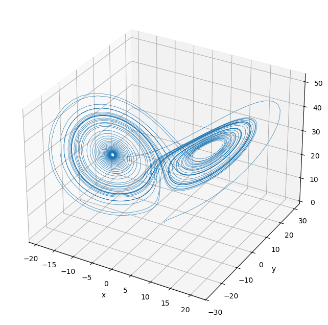
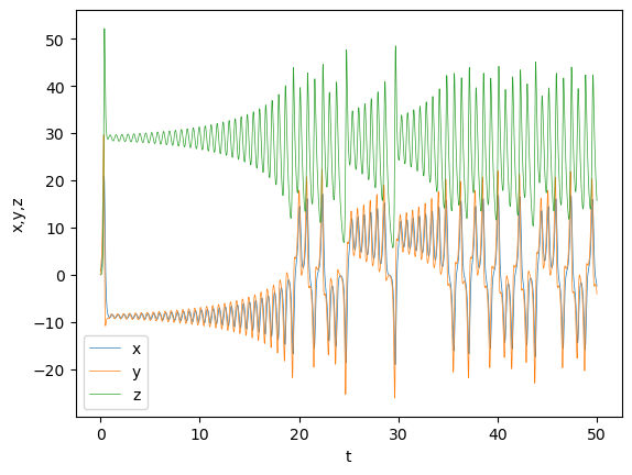
Lorenz attractor

Edward Lorenz derived a simplified equation describing the convection of atmosphere and found that it shows non-periodic oscillation.

\[ \frac{dx}{dt} = p(y - x) \]

\[ \frac{dy}{dt} = -xz + rx - y \]

\[ \frac{dz}{dt} = xy - bz \]

def lorenz(xyz, t, p=10., r=28., b=8./3):
    """Lorenz equation"""
    x, y, z = xyz
    dxdt = p*(y - x)
    dydt = -x*z + r*x - y
    dzdt = x*y - b*z
    return np.array([dxdt, dydt, dzdt])

y0 = np.array([1, 0, 0])
t = np.arange(0, 50, 0.01)
y = odeint(lorenz, y0, t, args=(10., 30., 8./3))
plt.plot(t, y, lw=0.5);
plt.xlabel('t'); plt.ylabel('x,y,z'); plt.legend(('x','y','z'));

# Uncomment below for interactive viewing
#%matplotlib widget

# Plot in 3D
fig = plt.figure(figsize=(8,8))
ax = fig.add_subplot(projection='3d')
ax.plot(y[:,0], y[:,1], y[:,2], lw=0.5);
plt.xlabel('x'); plt.ylabel('y'); ax.set_zlabel('z');