6. Ordinary Differential Equations: Exercise Solutions#
import numpy as np
import matplotlib.pyplot as plt
%matplotlib inline
from scipy.integrate import odeint
1. Linear ODEs#
Like the exponential of a real number \(x\) is given by $\( e^{x} = 1 + x + \frac{1}{2} x^2 + \frac{1}{6} x^3 + ... = \sum_{k=0}^{\infty} \frac{1}{k!} x^k, \)\( the *exponential of a matrix* \)X\( is defined as \)\( e^{X} = I + X + \frac{1}{2} X^2 + \frac{1}{6} X^3 + ... = \sum_{k=0}^{\infty} \frac{1}{k!} X^k. \)$
For one dimensional linear ODE $\( \frac{dy}{dt} = a y \)\( the solution is given by \)\( y(t) = e^{at} y(0), \)\( where \)y(0)$ is the initial state.
For an \(n\) dimensional linear ODE $\( \frac{dy}{dt} = A y \)\( where \)A\( is an \)n\times n\( matrix, the solution is given by the matrix exponential \)\( y(t) = e^{At} y(0), \)\( where \)y(0)\( is an \)n$-dimensional initial state.
Verify this by expanding \(e^{At}\) accordint to the definition and differentiating each term by \(t\).
The behavior of the matrix exponentioal \(e^{At}\) depends on the eivenvalues of \(A\); whether the eigenvalues are real or complex, and whether the real part is positive or negative.
Let us visualize solutions for different eigenvalues.
def linear(y, t, A):
    """Linear dynamcal system dy/dt = Ay
    y: n-dimensional state vector
    t: time (not used, for compatibility with odeint())
    A: n*n matrix"""
    # y is an array (row vector), A is a matrix
    return A@y
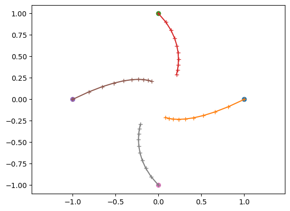
def linear2D(A, yinit=np.array([[1,0],[0,1],[-1,0],[0,-1]]), t=np.arange(0, 5, 0.1)):
    """Visualizing linear 2D dynamical system"""
    for y0 in yinit:
        y = odeint(linear, y0, t, args=(A,))
        plt.plot(y[0,0], y[0,1], 'o')   # starting point
        plt.plot(y[:,0], y[:,1], '+-')  # trajectory
    plt.axis('equal')
    return np.linalg.eig(A)
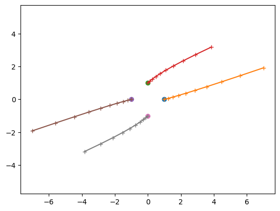
Real eigenvalues \(\lambda_1 > \lambda_2 > 0\)
A = np.array([[2, 1], [0.5, 1]])  # modift this!
linear2D(A, t=np.arange(0, 1, 0.1))
EigResult(eigenvalues=array([2.3660254, 0.6339746]), eigenvectors=array([[ 0.9390708 , -0.59069049],
       [ 0.34372377,  0.80689822]]))
Real eigenvalues \(\lambda_1 > 0 > \lambda_2\)
A = np.array([[2, 1], [0.5, -1]])
linear2D(A, t=np.arange(0, 1, 0.1))
EigResult(eigenvalues=array([ 2.1583124, -1.1583124]), eigenvectors=array([[ 0.98769933, -0.30185542],
       [ 0.15636505,  0.95335371]]))
Real eigenvalues \(0 > \lambda_1 > \lambda_2\)
A = np.array([[-2, 1], [0.5, -1]])
linear2D(A, t=np.arange(0, 1, 0.1))
EigResult(eigenvalues=array([-2.3660254, -0.6339746]), eigenvectors=array([[-0.9390708 , -0.59069049],
       [ 0.34372377, -0.80689822]]))
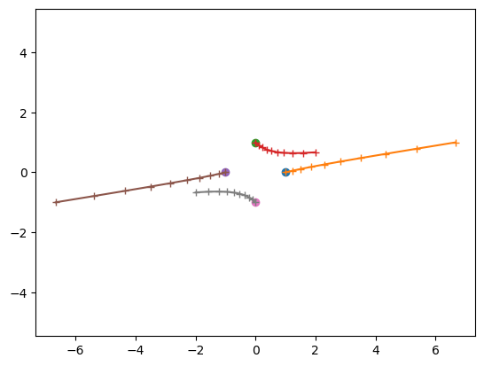
Complex eigenvalues \(\lambda_1=a+ib\) and \(\lambda_2=a-ib\) with \(a>0\)
A = np.array([[2, 2], [-1, 1]])
linear2D(A, t=np.arange(0, 1, 0.1))
EigResult(eigenvalues=array([1.5+1.32287566j, 1.5-1.32287566j]), eigenvectors=array([[ 0.81649658+0.j        ,  0.81649658-0.j        ],
       [-0.20412415+0.54006172j, -0.20412415-0.54006172j]]))
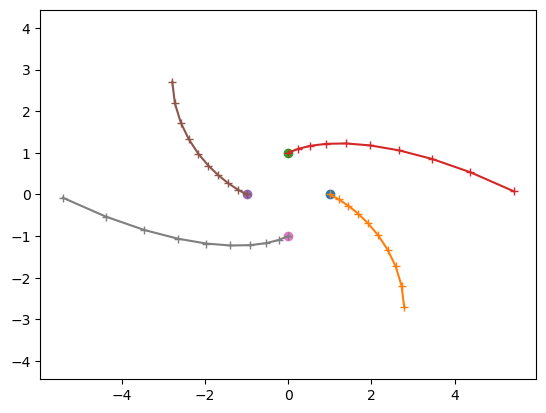
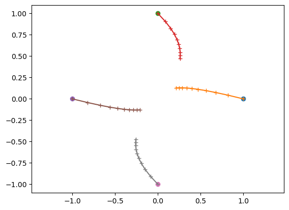
Complex eigenvalues \(\lambda_1=a+ib\) and \(\lambda_2=a-ib\) with \(a<0\)
A = np.array([[-2, 1], [-1, -1]])
linear2D(A, t=np.arange(0, 1, 0.1))
EigResult(eigenvalues=array([-1.5+0.8660254j, -1.5-0.8660254j]), eigenvectors=array([[0.70710678+0.j        , 0.70710678-0.j        ],
       [0.35355339+0.61237244j, 0.35355339-0.61237244j]]))
c.f. For a 2 by 2 matrix $\( A = \pmatrix{a & b \\ c & d}, \)\( we can analytically derive the eivenvalues from \)\( \det (A - \lambda I) = (a-\lambda)(d-\lambda) - bc = 0 \)\( as \)\( \lambda = \frac{a+d}{2} \pm \sqrt{\frac{(a-d)^2}{4}+ bc}. \)$
2. Nonlinear ODEs#
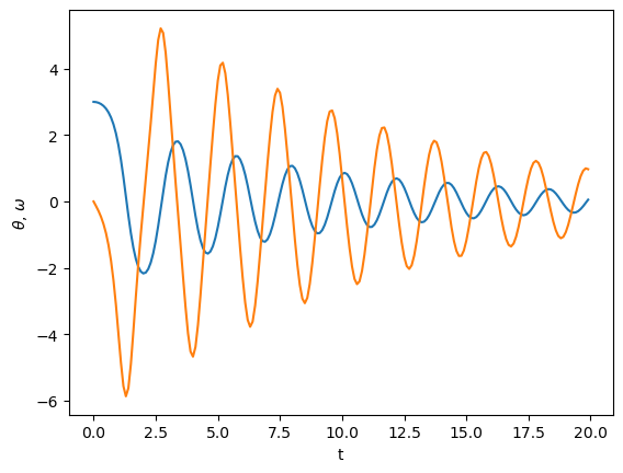
Implement a nonlinear system, such as a pendulum with friction \(\mu\): $\( \frac{d\theta}{dt} = \omega \)\( \)\( ml^2 \frac{d\omega}{dt} = - \mu \omega - mgl \sin \theta \)$
def pendulum(y, t, m=1, l=1, mu=0.1, g=9.8):
    th, om = y
    dthdt = om
    domdt = -(mu*om + m*g*l*np.sin(th))/(m*l*l)
    return [dthdt, domdt]
Run a simulation by
odeint()and show the trajectory as (t, y(t))
y0 = np.array([3, 0])
t = np.arange(0, 20, 0.1)
y = odeint(pendulum, y0, t, args=(1, 1, 0.2, 9.8))
plt.plot(t, y)  # trajectory
plt.xlabel('t'); plt.ylabel('$\\theta$, $\omega$');
<>:5: SyntaxWarning: invalid escape sequence '\o'
<>:5: SyntaxWarning: invalid escape sequence '\o'
/var/folders/dd/3kwwsm055d1cc1w134st1f580000gn/T/ipykernel_62061/284280705.py:5: SyntaxWarning: invalid escape sequence '\o'
  plt.xlabel('t'); plt.ylabel('$\\theta$, $\omega$');
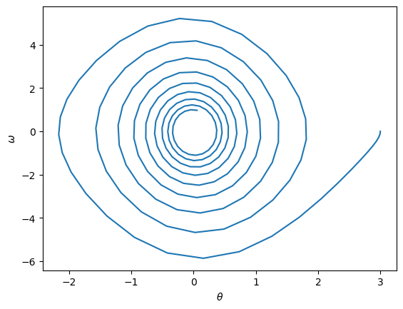
Show the trajectory in the 2D state space \((\theta, \omega)\)
plt.plot(y[:,0], y[:,1]);  # phase plot
plt.xlabel('$\\theta$'); plt.ylabel('$\omega$');
<>:2: SyntaxWarning: invalid escape sequence '\o'
<>:2: SyntaxWarning: invalid escape sequence '\o'
/var/folders/dd/3kwwsm055d1cc1w134st1f580000gn/T/ipykernel_62061/2133674605.py:2: SyntaxWarning: invalid escape sequence '\o'
  plt.xlabel('$\\theta$'); plt.ylabel('$\omega$');
Option) Implement a nonlinear system with time-dependent input, such as a forced pendulum: $\( \frac{d\theta}{dt} = \omega \)\( \)\( ml^2 \frac{d\omega}{dt} = - \mu \omega - mgl \sin\theta + a\sin bt\)$ and see how the behavior changes with the input.
3. Bifurcation#
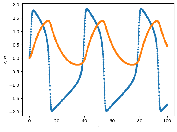
FitzHugh-Nagumo model is an extension of Van der Pol model to approximate spiking behaviors of neurons. $\( \frac{dv}{dt} = v - \frac{v^3}{3} - w + I \)\( \)\( \frac{dw}{dt} = \phi (v + a - bw) \)$
Implement a function and see how the behaviors at different input current \(I\).
def fhn(y, t, I=0, a=0.7, b=0.8, phi=0.08):
    """FitzHugh-Nagumo model"""
    v, w = y
    dvdt = v - v**3/3 - w + I
    dwdt = phi*(v + a -b*w)
    return np.array([dvdt, dwdt])
y0 = np.array([0, 0])
t = np.arange(0, 100, 0.1)
y = odeint(fhn, y0, t, args=(0.5,))
plt.plot(t, y, '.-')  # trajectory
plt.xlabel('t'); plt.ylabel('v, w');
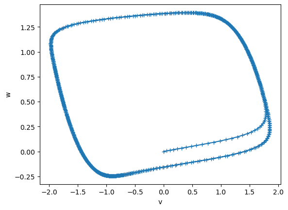
plt.plot(y[:,0], y[:,1], '+-')  # phase plot
plt.xlabel('v'); plt.ylabel('w');
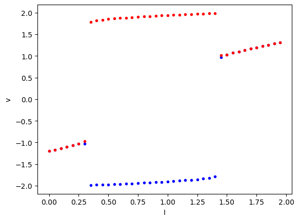
Draw a bifurcation diagram showing the max-min of \(v\) for different values of \(I\).
# bifurcation diagram
t = np.arange(0, 200, 0.1)
for I in np.arange(0., 2., 0.05):
    y = odeint(fhn, y0, t, args=(I,))  # change I
    plt.plot(I, min(y[1000:,0]), "b.")
    plt.plot(I, max(y[1000:,0]), "r.")
plt.xlabel('I'); plt.ylabel('v');