


4. Vectors and Matrices: Exercise Solutions#
import numpy as np
import matplotlib.pyplot as plt
%matplotlib inline
1) Determinant and eigenvalues#
For a 2x2 matrix \(A = \left(\begin{array}{cc} a & b\\ c & d \end{array}\right)\), let us verify that \(\det A = ad - bc\) in the case graphically shown below (\(a, b, c, d\) are positive).
A = np.array([[4, 1], [2, 3]])
plt.plot([0, 1, 1, 0, 0], [0, 0, 1, 1, 0])
plt.plot([0, A[0,0]+A[0,1], A[0,0]+A[0,1], 0, 0],
         [0, 0, A[1,0]+A[1,1], A[1,0]+A[1,1], 0])
plt.plot([A[0,0], A[0,0]+A[0,1], A[0,0]+A[0,1], A[0,0], A[0,0]],
         [0, 0, A[1,0], A[1,0], 0])
plt.plot([0, A[0,1], A[0,1], 0, 0],
         [A[1,1], A[1,1], A[1,0]+A[1,1], A[1,0]+A[1,1], A[1,1]])
plt.plot([0, A[0,0], A[0,0]+A[0,1], A[0,1], 0],
         [0, A[1,0], A[1,0]+A[1,1], A[1,1], 0])
plt.axis('equal')
plt.text(A[0,0], A[1,0], '(a,c)')
plt.text(A[0,1], A[1,1], '(b,d)')
plt.text(A[0,0]+A[0,1], A[1,0]+A[1,1], '(a+b,c+d)');
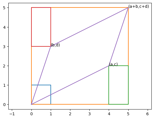
A unit square is transformed into a parallelogram. Its area \(S\) can be derived as follows:
Large rectangle: \( S_1 = (a+b)(c+d) = ac+ad+bc+bd \)
Small rectangle: \( S_2 = bc \)
Bottom/top triangle: \( S_3 = ac/2 \)
Left/right triangle: \( S_4 = bd/2 \)
Parallelogram:
$\( S = S_1 - 2S_2 - 2S_3 - 2S_4 = ad - bc\)$
The determinant equals the product of all eigenvalues. Verify this numerically for multiple cases and explain intuitively why that should hold.
#A = np.array([[1, 2], [3, 4]])
m = 4
A = np.random.randn(m,m)
print(A)
lam, V = np.linalg.eig(A)
print('eigenvalues = ', lam)
print('product = ', np.product(lam))
det = np.linalg.det(A)
print('detrminant = ', det)
[[-0.94415858  1.60569827  0.29823159 -0.50595799]
 [-1.13841117 -1.18249616 -0.31472788 -0.74692224]
 [ 0.61810412  0.09815888 -0.14378233  1.06800798]
 [ 1.99648672  0.34718984  0.58858848 -0.75195617]]
eigenvalues =  [-0.70436002+1.60308311j -0.70436002-1.60308311j -1.54531078+0.j
 -0.06836244+0.j        ]
product =  (0.32389578403514835-3.820896749682147e-18j)
detrminant =  0.32389578403514757
The determinant represents how much the volume in the original space is expanded or shrunk.
The eigenvalues represent how much a segment in the direction of eigen vector is scaled in length.
Therefore, the producs of all eigenvalues should equal to the determinant.
2) Eigenvalues and matrix product#
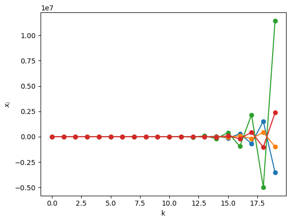
Make a random (or hand-designed) \(m\times m\) matrix \(A\). Compute its eigenvalues and eigenvectors. From a random (or your preferred) initial point \(\b{x}\), compute \(A\b{x}, A^2\b{x}, A^3\b{x},...\) and visualize the points. Then characterize the behavior of the points with respect the eigenvalues and eigenvectors.
m = 4
A = np.random.randn(m,m)
print('A = ', A)
L, V = np.linalg.eig(A)
print('eigenvalues = ', L)
#print('eigenvectors =\n', V)
A =  [[ 0.14028547 -0.60534656  0.60997173  0.42556625]
 [ 0.23783496  0.67662317  0.03224008  1.43861564]
 [ 0.07235662  0.36246447 -2.17005992 -0.34235269]
 [ 1.11382383  1.31910517  0.07533941 -0.45219159]]
eigenvalues =  [ 1.40226842  0.60603414 -1.51884655 -2.29479888]
# take a point and see how it moves
K = 20  # steps
x = np.zeros((m, K))
x[:,0] = np.random.randn(m) # random initial state
for k in range(K-1):
    x[:,k+1] = A @ x[:,k]  # x_{k+1} = A x_k
# plot the trajectory
plt.plot( x.T, 'o-')
plt.xlabel("k"); plt.ylabel("$x_i$");
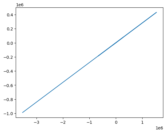
plt.plot( x[0,:], x[1,:])
[<matplotlib.lines.Line2D at 0x12a2c70b0>]
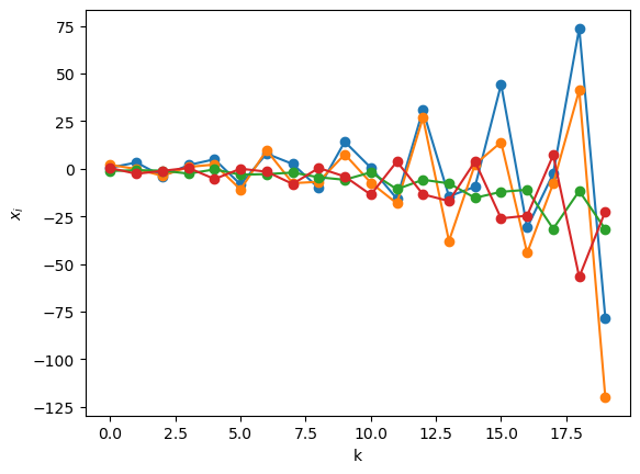
Do the above with several different matrices
A = np.random.randn(m,m)
print('A = ', A)
L, V = np.linalg.eig(A)
print('eigenvalues = ', L)
for k in range(K-1):
    x[:,k+1] = A @ x[:,k]  # x_{k+1} = A x_k
# plot the trajectory
plt.plot( x.T, 'o-')
plt.xlabel("k"); plt.ylabel("$x_i$");
A =  [[-0.69649275  0.40499098 -2.10710374  1.1993998 ]
 [ 0.19195423 -0.84012932 -0.68676938  1.88999116]
 [ 0.56803283 -0.34862034  0.61751071  0.91490006]
 [-0.30080831 -0.13707271  1.75801106 -0.45648666]]
eigenvalues =  [ 1.20168046+0.j         -0.70971525+0.94705015j -0.70971525-0.94705015j
 -1.15784796+0.j        ]
3) Principal component analysis#
Read in the “digits” dataset, originally from sklearn.
data = np.loadtxt("data/digits_data.txt")
target = np.loadtxt("data/digits_target.txt", dtype='int64')
m, n = data.shape
print(m, n)
1797 64
The first ten samples look like these:
plt.figure(figsize=(10,4))
for i in range(10):
    plt.subplot(1,10,i+1)
    plt.imshow(data[i].reshape((8,8)))
    plt.title(target[i])
    plt.axis('off')

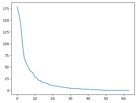
Compute the principal component vectors from all the digits and plot the eigenvalues from the largest to smallest.
# subtract the mean
Xm = np.mean(data, axis=0)
X = data - Xm
#C = np.cov(X, rowvar=False)
C = (X.T @ X)/(m-1)
lam, V = np.linalg.eig(C)
# columns of V are eigenvectors
# it is not guaranteed that the eigenvalues are sorted, so sort them
ind = np.argsort(-lam)  # indices for sorting, descending order
L = lam[ind]
V = V[:,ind]
print('L, V = ', L, V)
plt.plot(L);
L, V =  [1.79006930e+02 1.63717747e+02 1.41788439e+02 1.01100375e+02
 6.95131656e+01 5.91085249e+01 5.18845391e+01 4.40151067e+01
 4.03109953e+01 3.70117984e+01 2.85190412e+01 2.73211698e+01
 2.19014881e+01 2.13243565e+01 1.76367222e+01 1.69468639e+01
 1.58513899e+01 1.50044602e+01 1.22344732e+01 1.08868593e+01
 1.06935663e+01 9.58259779e+00 9.22640260e+00 8.69036872e+00
 8.36561190e+00 7.16577961e+00 6.91973881e+00 6.19295508e+00
 5.88499123e+00 5.15586690e+00 4.49129656e+00 4.24687799e+00
 4.04743883e+00 3.94340334e+00 3.70647245e+00 3.53165306e+00
 3.08457409e+00 2.73780002e+00 2.67210896e+00 2.54170563e+00
 2.28298744e+00 1.90724229e+00 1.81716569e+00 1.68996439e+00
 1.40197220e+00 1.29221888e+00 1.15893419e+00 9.31220008e-01
 6.69850594e-01 4.86065217e-01 2.52350432e-01 9.91527944e-02
 6.31307848e-02 6.07377581e-02 3.96662297e-02 1.49505636e-02
 8.47307261e-03 3.62365957e-03 1.27705113e-03 6.61270906e-04
 4.12223305e-04 0.00000000e+00 0.00000000e+00 0.00000000e+00] [[ 0.          0.          0.         ...  1.          0.
   0.        ]
 [ 0.01730947  0.01010646 -0.01834207 ...  0.          0.
   0.        ]
 [ 0.22342883  0.04908492 -0.12647554 ...  0.          0.
   0.        ]
 ...
 [ 0.08941847 -0.17669712 -0.23208416 ...  0.          0.
   0.        ]
 [ 0.03659771 -0.01945471 -0.16702656 ...  0.          0.
   0.        ]
 [ 0.0114685   0.00669694 -0.03480438 ...  0.          0.
   0.        ]]
# use SVD
U, S, Vt = np.linalg.svd(X, full_matrices=False)
# columns of V, or rows of Vt are eigenvectors
L = S**2/(m-1)  # eigenvalues
print('L, Vt = ', L, Vt)
plt.plot(L);
L, Vt =  [1.79006930e+02 1.63717747e+02 1.41788439e+02 1.01100375e+02
 6.95131656e+01 5.91085249e+01 5.18845391e+01 4.40151067e+01
 4.03109953e+01 3.70117984e+01 2.85190412e+01 2.73211698e+01
 2.19014881e+01 2.13243565e+01 1.76367222e+01 1.69468639e+01
 1.58513899e+01 1.50044602e+01 1.22344732e+01 1.08868593e+01
 1.06935663e+01 9.58259779e+00 9.22640260e+00 8.69036872e+00
 8.36561190e+00 7.16577961e+00 6.91973881e+00 6.19295508e+00
 5.88499123e+00 5.15586690e+00 4.49129656e+00 4.24687799e+00
 4.04743883e+00 3.94340334e+00 3.70647245e+00 3.53165306e+00
 3.08457409e+00 2.73780002e+00 2.67210896e+00 2.54170563e+00
 2.28298744e+00 1.90724229e+00 1.81716569e+00 1.68996439e+00
 1.40197220e+00 1.29221888e+00 1.15893419e+00 9.31220008e-01
 6.69850594e-01 4.86065217e-01 2.52350432e-01 9.91527944e-02
 6.31307848e-02 6.07377581e-02 3.96662297e-02 1.49505636e-02
 8.47307261e-03 3.62365957e-03 1.27705113e-03 6.61270906e-04
 4.12223305e-04 1.14286697e-30 1.14286697e-30 1.12542605e-30] [[ 1.77484909e-19  1.73094651e-02  2.23428835e-01 ...  8.94184677e-02
   3.65977111e-02  1.14684954e-02]
 [-3.27805401e-18  1.01064569e-02  4.90849204e-02 ... -1.76697117e-01
  -1.94547053e-02  6.69693895e-03]
 [ 1.68358559e-18 -1.83420720e-02 -1.26475543e-01 ... -2.32084163e-01
  -1.67026563e-01 -3.48043832e-02]
 ...
 [ 0.00000000e+00  8.62555218e-17  2.89406017e-17 ...  1.11022302e-16
   1.11022302e-16 -3.26128013e-16]
 [ 0.00000000e+00 -5.34891730e-16  4.27024926e-17 ...  0.00000000e+00
   8.32667268e-17 -1.04083409e-16]
 [-1.00000000e+00  1.68983002e-17 -5.73338351e-18 ... -8.66631300e-18
   1.57615962e-17 -4.07058917e-18]]
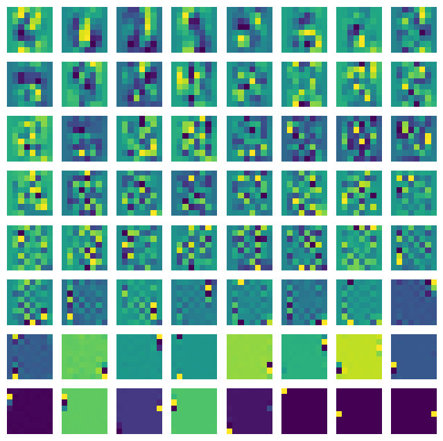
Visualize the principal vectors as images.
plt.figure(figsize=(8,8))
for i in range(n):
    plt.subplot(8,8,i+1)
    plt.imshow(V[:,i].reshape((8,8)))
    #plt.imshow(Vt[i].reshape((8,8)))
    plt.axis('off')
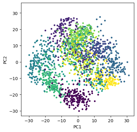
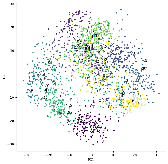
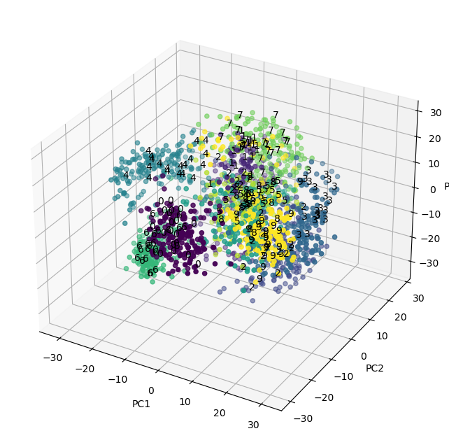
Scatterplot the digits in the first two or three principal component space, with different colors/markers for digits.
# columns of V are eigenvectors
Z = X @ V
plt.scatter(Z[:,0], Z[:,1], c=target, marker='.')
plt.setp(plt.gca(), xlabel='PC1', ylabel='PC2')
plt.axis('square');
plt.figure(figsize=(8,8))
plt.scatter(Z[:,0], Z[:,1], c=target, marker='.')
# add labels to some points
for i in range(100):
    plt.text(Z[i,0], Z[i,1], str(target[i]))
plt.setp(plt.gca(), xlabel='PC1', ylabel='PC2');
# In 3D
fig = plt.figure(figsize=(8,8))
ax = fig.add_subplot(projection='3d')
ax.scatter(Z[:,0], Z[:,1], Z[:,2], c=target, marker='o')
# add labels to some points
for i in range(200):
    ax.text(Z[i,0], Z[i,1], Z[i,2], str(target[i]))
plt.setp(plt.gca(), xlabel='PC1', ylabel='PC2', zlabel='PC3');
Take a sample digit, decompose it into principal components, and reconstruct the digit from the first \(m\) components. See how the quality of reproduction depends on \(m\).
K = 8  # PCs to be considered
i = np.random.randint(m) # pick a random sample
plt.figure(figsize=(10,4))
plt.subplot(1,K,1)
plt.imshow(data[i].reshape((8,8))) # original
plt.title(target[i])
plt.axis('off')
for k in range(1,K):  # number of PCs
    Xrec = Xm + V[:,:k] @ Z[i,:k]
    plt.subplot(1,K,k+1)
    plt.imshow(Xrec.reshape((8,8))) # reconstructed
    plt.title(k)
    plt.axis('off')
