Real and Complex Eigenvalues

\[ % Latex macros \newcommand{\mat}[1]{\begin{pmatrix} #1 \end{pmatrix}} \newcommand{\p}[2]{\frac{\partial #1}{\partial #2}} \newcommand{\b}[1]{\boldsymbol{#1}} \newcommand{\w}{\boldsymbol{w}} \newcommand{\x}{\boldsymbol{x}} \newcommand{\y}{\boldsymbol{y}} \]

import numpy as np
import matplotlib.pyplot as plt
%matplotlib inline

Eigenvalues of a 2x2 matrix

Let us take the simplest and the most important case of 2 by 2 matrix

\[\begin{split} A = \pmatrix{a & b \\ c & d}. \end{split}\]

We can analytically derive the eigenvalues from

\[ \det (A - \lambda I) = (a-\lambda)(d-\lambda) - bc = 0 \]

as

\[ \lambda = \frac{a+d}{2} \pm \sqrt{\frac{(a-d)^2}{4}+ bc}. \]

The corresponding eigenvectors are not unique, but given by, for example,

\[\begin{split} \b{x} = \mat{b \\ \lambda - a}. \end{split}\]

Real eigenvalues

When \(\frac{(a-d)^2}{4}+ bc \ge 0\), \(A\) has two real eigenvalues \(\{\lambda_1, \lambda_2\}\) with corresponding eigenvectors \(\{ \b{v}_1, \b{v}_2 \}\)

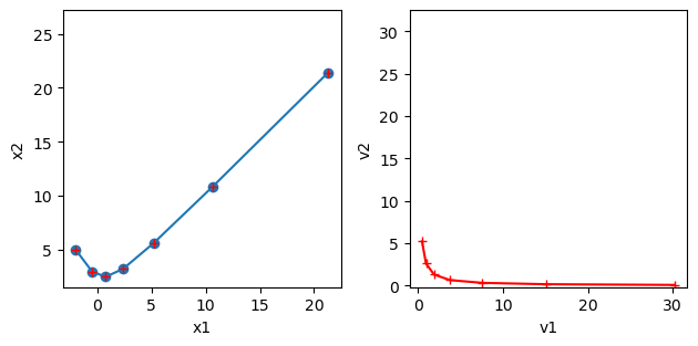
The movement of a point \(\b{x}\) by \(A\) as \(A\b{x}, A^2\b{x}, A^3\b{x},...\) is composed of movements in the directions of the eigenvectors \(\{ \b{v}_1, \b{v}_2 \}\). It is convergent if \(|\lambda_i|<1\) and divergent if \(|\lambda_i|>1.\)

# take a 2x2 matrix
A = np.array([[1.5, 0.5], [1, 1]])
# check the eigenvalues and eigenvectors
L, V = np.linalg.eig(A)
print("L =", L)
print("V = ", V)
# take a point and see how it moves
K = 7  # steps
x = np.zeros((2, K))
x[:,0] = [-2, 5]
for k in range(K-1):
    x[:,k+1] = A @ x[:,k]  # x_{k+1} = A x_k
# plot the trajectory
plt.subplot(1,2,1)
plt.plot( x[0], x[1], 'o-')
plt.axis('square'); plt.xlabel("x1"); plt.ylabel("x2");
# In the eigenspace
y = np.zeros((2, K))
y[:,0] = np.linalg.inv(V) @ x[:,0] # map to eigenspace
for k in range(K-1):
    y[:,k+1] = L*y[:,k]  # z_{k+1} = L z_k
plt.subplot(1,2,2)
plt.plot( y[0], y[1], 'r+-')
plt.axis('square'); plt.xlabel("v1"); plt.ylabel("v2");
# Convert back to the original space
plt.subplot(1,2,1)
xv = (V @ y).real
plt.plot( xv[0], xv[1], 'r+')
plt.tight_layout();  # adjust the space

L = [2.  0.5]
V =  [[ 0.70710678 -0.4472136 ]
 [ 0.70710678  0.89442719]]

Complex eigenvalues

When \(\frac{(a-d)^2}{4}+ bc < 0\), \(A\) has a pair of complex eigenvalues

\[ \lambda_1 = \alpha + i\beta \mbox{ and } \lambda_2 = \alpha - i\beta \]

where

\[ \alpha = \frac{a+d}{2} \mbox{ and } \beta^2 = -\frac{(a-d)^2}{4}- bc \]

with corresponding eigenvectors

\[ V = (\b{v}_1, \b{v}_2) = (\b{u}+i\b{w}, \b{u}-i\b{w}).\]

By eigendecomposition \( A = V \Lambda V^{-1}, \) a point \(\b{x}\) is converted to points in a complex plane and multiplied by a complex eigenvalue, which means rotation and scaling. Points in the complex plane are then converted back in a real vector space by multiplication with \(V\).

To see the rotation and scaling more explicitly, we can represent \(\Lambda=\mat{\alpha+i\beta & 0 \\ 0 & \alpha-i\beta}\) as

\[\Lambda = U R U^{-1}\]

where \(R\) is

\[\begin{split} R = \mat{\alpha & -\beta \\ \beta & \alpha} = \mat{r\cos\theta & -r\sin\theta \\ r\sin\theta & r\cos\theta }.\end{split}\]

Here \(r=|\lambda|=\sqrt{\alpha^2+\beta^2}\) is the scaling factor and \(\theta\) is the angle of rotation.

We can choose \(U\) as

\[\begin{split} U = \frac{1}{2}\mat{1 & i \\ 1 & -i} \end{split}\]

such that \(VU = (\b{u}, -\b{w})\).

Then we have another decomposition of \(A\) as

\[\begin{split} A = V \Lambda V^{-1} = V URU^{-1} V^{-1} = (\b{u}, -\b{w}) \mat{r\cos\theta & -r\sin\theta \\ r\sin\theta & r\cos\theta} (\b{u}, -\b{w})^{-1} \end{split}\]

# take a 2x2 matrix
A = np.array([[1, -1], [1, 0.5]])
# check the eigenvalues and eigenvectors
L, V = np.linalg.eig(A)
print("L =", L)
print("V = ", V)
# take a point and see how it moves
K = 7  # steps
x = np.zeros((2, K))
x[:,0] = [1, 0]
for k in range(K-1):
    x[:,k+1] = A @ x[:,k]  # x_{k+1} = A x_k
# plot the trajectory
plt.subplot(1,3,1)
plt.plot( x[0], x[1], 'o-')
plt.axis('square'); plt.xlabel("x1"); plt.ylabel("x2");
# In the eigenspace
z = np.zeros((2, K), dtype=complex)
z[:,0] = np.linalg.inv(V) @ x[:,0]
for k in range(K-1):
    z[:,k+1] = L*z[:,k]  # z_{k+1} = L z_k
plt.subplot(1,3,2)
plt.plot( z[0].real, z[0].imag, 'r+-')
plt.plot( z[1].real, z[1].imag, 'm+-')
plt.axis('square'); plt.xlabel("Real"); plt.ylabel("Imag");
# In the cos-sin space
VU = np.c_[V[:,0].real, -V[:,0].imag]
R = np.array([[L[0].real, -L[0].imag], [L[0].imag, L[0].real]])
print("R =", R)
print("VU =", VU) 
y = np.zeros((2, K))
y[:,0] = np.linalg.inv(VU) @ x[:,0]
for k in range(K-1):
    y[:,k+1] = R @ y[:,k]  # y_{k+1} = R y_k
plt.subplot(1,3,3)
plt.plot( y[0], y[1], 'g*-')
plt.axis('square'); plt.xlabel("u"); plt.ylabel("-w");
# Convert back to the original space
plt.subplot(1,3,1)
xc = (V @ z).real
xr = VU @ y
plt.plot( xr[0], xr[1], 'g*')
plt.plot( xc[0], xc[1], 'r+')
plt.tight_layout(rect=[0, 0, 1.5, 1]);  # fit in extra width

L = [0.75+0.96824584j 0.75-0.96824584j]
V =  [[0.70710678+0.j        0.70710678-0.j       ]
 [0.1767767 -0.6846532j 0.1767767 +0.6846532j]]
R = [[ 0.75       -0.96824584]
 [ 0.96824584  0.75      ]]
VU = [[ 0.70710678 -0.        ]
 [ 0.1767767   0.6846532 ]]

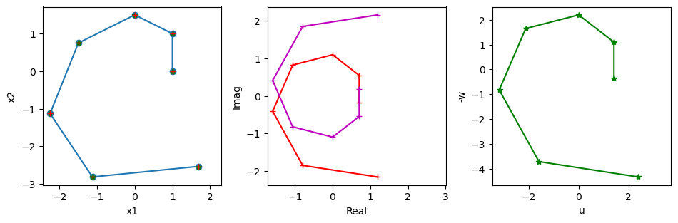
The trajectory in the complex space or the \((\b{u},-\b{w})\) space is a regular spirals, which is mapped to a skewed spiral in the original space.