Custom time distributions (using pure R)

Introduction

NEXTNetR provides a set of built-in time distributions that can be used as transmission and recovery times in simulations, see help(time_distributions). Additional distributions can be defined by users through either R or C++ code. Here we discuss the simpler but much (order of magnitude!) slower R solution. See vignette("custom_time_distributions_cpp") for the faster but more complex C++ solution.

Loading the NEXTNetR package

We start with loading the NEXTNetR package. If the package is not already installed, see the website for installation instructions. We also load the ggplot2 and ggpubr packages for plotting and set a nice theme.

library(NEXTNetR)
library(ggplot2)
library(ggpubr)
theme_set(theme_pubr())

Implementing a custom time distribution in pure R

To implement a custom time distribution, we use userdefined_time(). This function allows us to provide arbitrary R functions that implement the functions listed in help(time_functions) for our distribution. Each function must take either a single argument tau or three arguments tau, t and m. At least two functions survival and density must be provided. by providing single-argument functions, we signal to NEXTNet that we only implement the base distribution and leave it to NEXTNet to derive the conditioned and modulated version of the distribution from that, see discussions in help(time_functions) and help(userdefined_time).

We use userdefined_time() to create a function mixture_time which returns a mixture of the distributions listed in times with weights weights.

mixture_time <- function(times, weights) {
  ud_time <- NULL
  ud_time <- userdefined_time(
    survival=function(tau)
      sum(sapply(times, time_survivalprobability, tau) * weights),
    density=function(tau)
      sum(sapply(times, time_density, tau) * weights),
    sample=function() {
      i <- sample.int(n=length(weights), prob = weights, size=1)
      return(time_sample(1, times[[i]]))
    },
  )
}

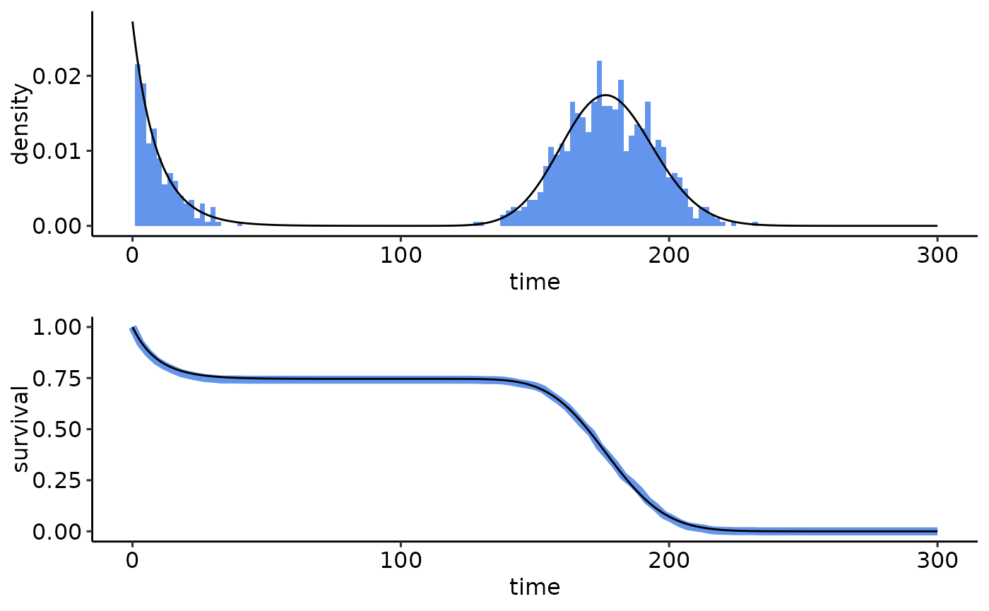
We now use the newly created mixture_time function to create a mixture of an exponential distribution with mean 5 and a log-normal distribution with mean 200 and variance 500, weighted so that 30% of samples come from the exponential distribution.

psi <- mixture_time(times=list(exponential_time(1/10),
                    lognormal_time(200, 500)), weights=c(0.3, 0.7))

To test this we sample from the newly created distribution using time_sample

samples <- time_sample(1e3, psi, t=10, m=2)

and use time_density and time_survivalprobability to compare the distribution of our samples (in blue) to the theoretical distribution (in black) to check that everything works correctly

samples.ecdf <- ecdf(samples)
ggarrange(
  ggplot() +
    lims(x=c(0, 300)) +
    geom_histogram(data=data.frame(time=samples),
                   aes(x=time, y=after_stat(density)),
                   binwidth=2, fill="cornflowerblue") +
    geom_function(fun=time_density, n=1000,
                  args=list(timedistribution=psi, t=10, m=2)),
  ggplot() +
    lims(x=c(0, 300), y=c(0,1)) + labs(x='time', y='survival') +
    geom_function(fun=function(x) 1 - samples.ecdf(x),
                  color="cornflowerblue", linewidth=2) +
    geom_function(fun=time_survivalprobability, n=1000,
                  args=list(timedistribution=psi, t=10, m=2)),
  ncol=1
)

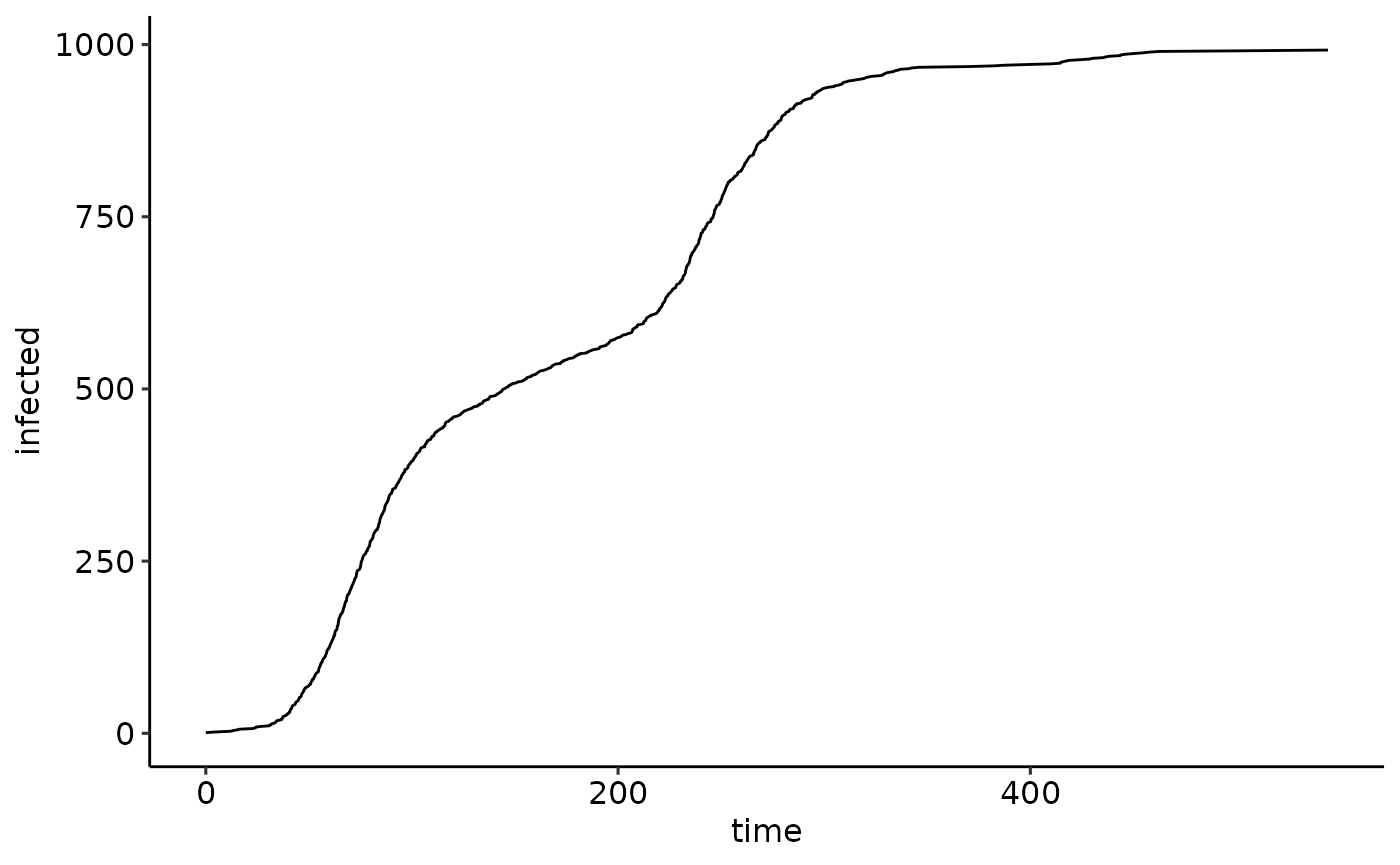
Simulations using our custom distribution

Our custom distribution in simulations in the same way as built-in distributions, see vignette("NEXTNetR") for a step by step explanation of this

nw <- erdos_renyi_network(1e3, 5)
sim <- simulation(nw, psi)
simulation_addinfections(sim, nodes=c(1), times=c(0.0))
events <- simulation_run(sim, stop=list(total_infected=300e3))
ggplot(events) +
  geom_line(aes(x=time, y=infected))