Custom time distributions (using C++)

Introduction

NEXTNetR provides a set of built-in time distributions that can be used as transmission and recovery times in simulations, see help(time_distributions). Additional distributions can be defined by users through either R or C++ code. Here we discuss the C++ solution, which is significantly (orders of magnitudes!) faster, but more complex. For the slower but simpler pure R solution, see vignette("custom_time_distributions_r").

Loading the NEXTNetR package

We start with loading all required packages. If NEXTNetRis not already installed, see the website for installation instructions. To conveniently mix C++ and R code, we use the cpp11 package together with decor. To implement a new distribution, our C++ code must be able to see global symbols related to the transmission_time class defined by the NEXTNetR package. Unfortunately, R packages are usually loaded in a way that prevents this. To work around this, we therefore have to load NEXTNetR’s shared library manually before importing the package. That way, we can specify local=TRUE when we load the library to make symbols globally visible. Note that this may not be required on all platforms. Finally, we also load the ggplot2 and ggpubr packages for plotting and set a nice theme.

# Make sure the NEXTNetR shared library is loaded with local=FALSE
# This has to be done *before* library(NEXTNetR)
nnR.dir <- find.package("NEXTNetR")
nnR.lib <- if (nzchar(.Platform$r_arch)) {
  file.path(nnR.dir, "libs", .Platform$r_arch,
            paste0("NEXTNetR", .Platform$dynlib.ext))
} else {
  file.path(nnR.dir, "libs",
            paste0("NEXTNetR", .Platform$dynlib.ext))
}
dyn.load(nnR.lib, local=FALSE, now=TRUE)

# Now we may load NEXTNetR
library(NEXTNetR)

# For cpp_source()
library(cpp11)
library(decor)

# For plotting
library(ggplot2)
library(ggpubr)
theme_set(theme_pubr())

Implementing a custom time distribution in C++

To implement a custom time distribution, we have to implement the time_distribution interface (i.e. abstract base class) defined by the NEXTNet C++ library. The minimal set of functions an implementation of that interface must provide are

virtual double density(interval_t tau) const;
virtual double survivalprobability(interval_t tau) const;

If only these two functions are provided, random samples of your distribution will be generated by generating a uniformly distribution random value between 0 and 1 and computing the corresponding quantile. Since we have not override the quantile function, the quantile will be computed by numerically inverting the survival function using bisection, which is slow. If there is a more efficient way of generating samples, you will thus want to also override the sample function

virtual interval_t sample(rng_t &, interval_t t, double m) const;

This function must sample from the derived distribution conditioned on \(t\) and modulated with \(m\), see help(time_functions) for a discussion of these parameters. Often, generating samples from the unmodified distribution, i.e. for \(t=0\) and \(m=1\) is considerably simpler. Since this is, on unweighted networks, also by far the most common case, a typical strategy is to only optimize this case, i.e. to do

virtual interval_t sample(rng_t &rng, interval_t t, double m) const override {
  if ((t == 0.0) && (m == 1.0)) {
    // generate sample from base distribution
    return ...
  }
  // Use numeric inversion of the survival function for the general case
  return transmission_time::sample(rng, t, m);
}

Finally, if the quantiles can be computed more efficiently than be inverting the survival function, also override the quantile function

virtual interval_t survivalquantile(double u) const;

A mixture of existing distributions

The following file mixture_time.cpp implements a mixture of \(n\) arbitrary time distributions with given weights. It defines a class mixture_time_impl which derives from the abstract base class time_distribution and implements the sample, survivalprobability, and density methods. To create mixture distributions, it provides a function mixture_time which converts the parameters appropriately and returns an instance of the mixture_time_impl as a transmission_time_R (this type encapsulates C++ time distribution objects so that they can be passed through R).

/* mixture_time.cpp */

#include <random>
#include <cpp11.hpp>
#include <cpp11/function.hpp>

#include "NEXTNetR/NEXTNetR_types.h"
#include "nextnet/random.h"

using namespace cpp11;

struct mixture_time_impl : public virtual transmission_time {
  virtual interval_t sample(rng_t &rng, interval_t t, double m) const override {
    if ((t == 0.0) && (m == 1.0))
      return times.at(pick(rng)).get()->sample(rng, 0.0, 1.0);
    return transmission_time::sample(rng, t, m);
  }
  
  virtual double survivalprobability(interval_t tau) const override {
    double p = 0.0;
    for(std::size_t i=0; i < times.size(); ++i)
      p += weights.at(i) * times.at(i).get()->survivalprobability(tau);
    return p;
  }

  virtual double density(interval_t tau) const override {
    double p = 0.0;
    for(std::size_t i=0; i < times.size(); ++i)
      p += weights.at(i) * times.at(i).get()->density(tau);
    return p;
  }
  std::vector<transmission_time_R> times;
  std::vector<double> weights;
  mutable std::discrete_distribution<std::size_t> pick;
};

[[cpp11::linking_to("BH")]]
[[cpp11::linking_to("NEXTNetR")]]
[[cpp11::register]]
SEXP mixture_time(list times, doubles weights) {
  // Validate parameters
  if (times.size() != weights.size())
    throw std::runtime_error("number of distributions and weights must agree");

  // Create object
  auto r = std::make_unique<mixture_time_impl>();
  
  // Set individual distributions and weights
  r->times.reserve(times.size());
  r->weights.reserve(times.size());
  double ws = 0.0;
  for(R_xlen_t i=0; i < times.size(); ++i)
      ws += weights[i];
  for(R_xlen_t i=0; i < times.size(); ++i) {
    r->times.push_back((transmission_time_R)times[i]);
    r->weights.push_back(weights[i] / ws);
  }
  r->pick = std::discrete_distribution<std::size_t>(
      weights.begin(), weights.end());

  // Return created object
  return transmission_time_R(r.release());
}

We could now compile this function externally and load the resulting shared library into R. However, cpp11 provides as simpler way in the form of the cpp_source() function. This function takes care of compiling, linking and loading the code, and makes all functions marked with [[cpp11::register]] available to R.

cpp_source('mixture_time.cpp', dir="/tmp/test", clean=FALSE, cxx_std="CXX17")

We can now use mixture_time as we would use any of the other distributions provided by NEXTNetR. For example, to create a mixture of an exponential distribution with mean 5 and a log-normal distribution with mean 200 and variance 500, weighted so that 30% of samples come from the exponential distribution, we can do

psi <- mixture_time(times=list(exponential_time(1/10),
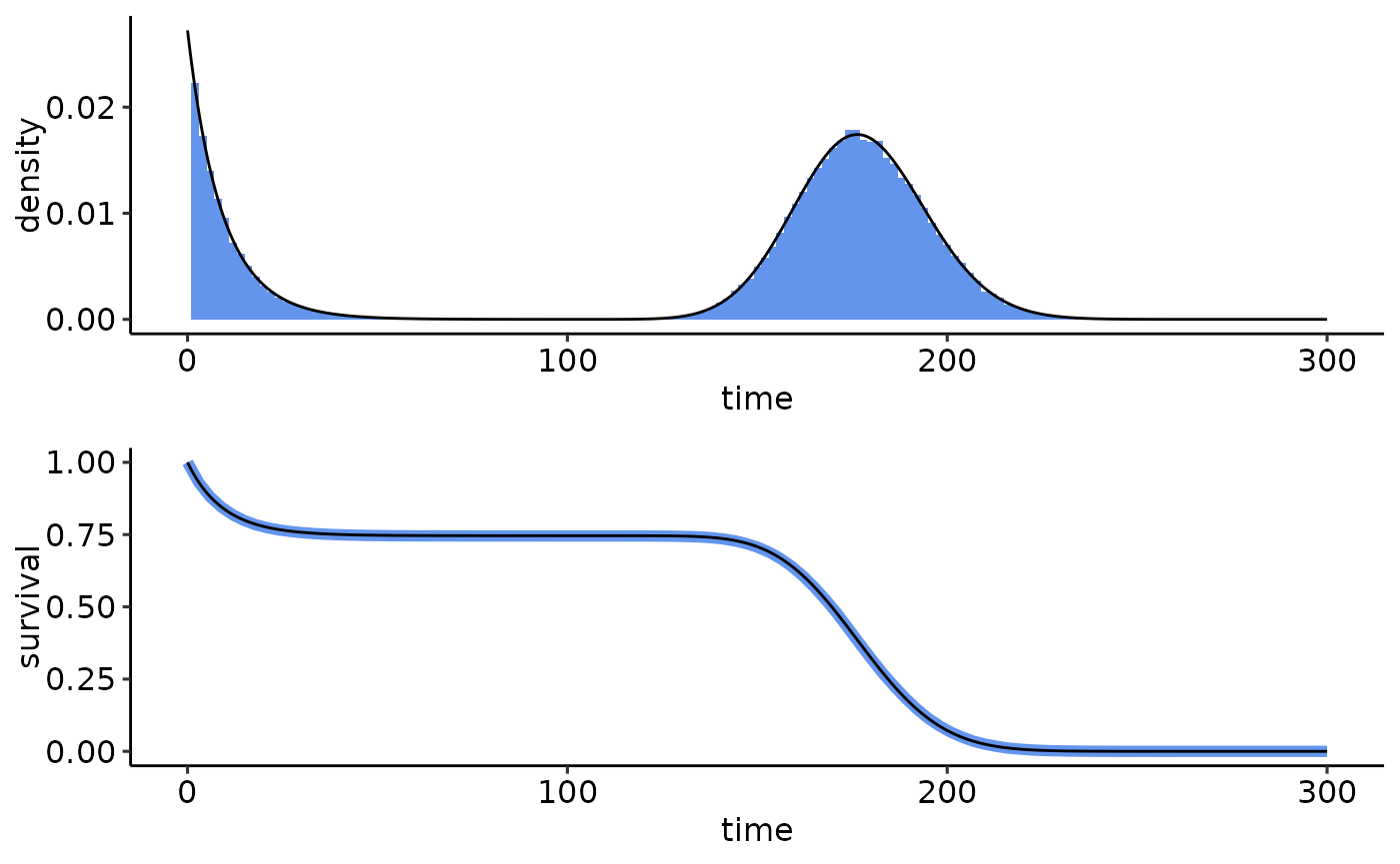
                    lognormal_time(200, 500)), weights=c(0.3, 0.7))

To test this we sample from the newly created distribution using time_sample

samples <- time_sample(1e5, psi, t=10, m=2)

and use time_density and time_survivalprobability to compare the distribution of our samples (in blue) to the theoretical distribution (in black) to check that everything works correctly

samples.ecdf <- ecdf(samples)
ggarrange(
  ggplot() +
    lims(x=c(0, 300)) +
    geom_histogram(data=data.frame(time=samples),
                   aes(x=time, y=after_stat(density)),
                   binwidth=2, fill="cornflowerblue") +
    geom_function(fun=time_density, n=1000,
                  args=list(timedistribution=psi, t=10, m=2)),
  ggplot() +
    lims(x=c(0, 300), y=c(0,1)) + labs(x='time', y='survival') +
    geom_function(fun=function(x) 1 - samples.ecdf(x),
                  color="cornflowerblue", linewidth=2) +
    geom_function(fun=time_survivalprobability, n=1000,
                  args=list(timedistribution=psi, t=10, m=2)),
  ncol=1
)

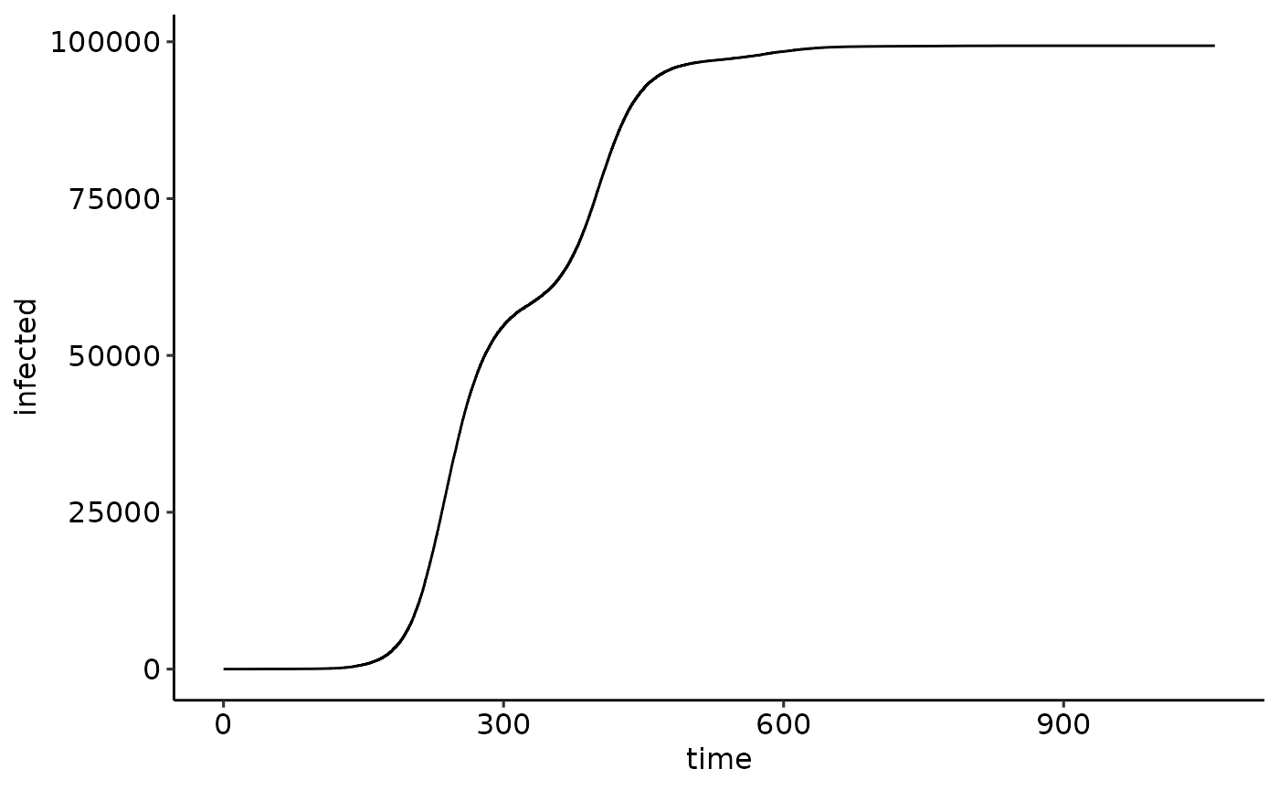
Simulations using our custom distribution

Our custom distribution in simulations in the same way as built-in distributions, see vignette(NEXTNetR) for a step by step explanation of this

nw <- erdos_renyi_network(1e5, 5)
sim <- simulation(nw, psi)
simulation_addinfections(sim, nodes=c(1), times=c(0.0))
events <- simulation_run(sim, stop=list(total_infected=300e3))
ggplot(events) +
  geom_line(aes(x=time, y=infected))