Basic Simulations of Epidemics • NEXTNetR

Loading the NEXTNetR package

We start with loading the NEXTNetR package. If the package is not already installed, see the website for installation instructions. We also load the ggplot2 and ggpubr packages for plotting and set a nice theme.

library(NEXTNetR)
library(ggplot2)
library(ggpubr)
theme_set(theme_pubr())

Creating and inspecting networks

Next we create a network object. To see the full list of network types supported by NEXTNetR, type help(network_types). Here, we create a random Erdős–Rényi network of a given size, i.e. with a given number of nodes. On Erdős–Rényi networks, each possible link has an probability to exist independent of all other links. This probability is computed such that nodes have the specified average degree (i.e. number of neighbours).

nw <- erdos_renyi_network(size=1e5, avg_degree=5)

The object nw now represents a specific network. We can inspect the network using the functions listed in help(network_properties). For example, we can query the number of neighbours of node 371 with

degree <- network_outdegree(nw, 371)
print(degree)
#> [1] 6

and knowing the degree we can query all neighbours of node 371.

network_neighbour(nw, 371, 1:degree)
#> [1] 18386 32383 63810 66115 83635 88963

Most inspection functions are vectorized and can query multiple nodes at once. For example, to plot the degree distribution as a histogram and compare it with the theoretically predicted Poisson distribution (dashed blue line) we can simply do

N <- network_size(nw)
ggplot(data.frame(degree=network_outdegree(nw, 1:N))) +
  geom_histogram(aes(x=degree, y=after_stat(count)),
                 binwidth=1, fill='darkgrey', color=NA) +
  geom_function(fun=function(n) N * dpois(round(n), 5),
                n=1000, color='blue', linetype="dashed", linewidth=0.5)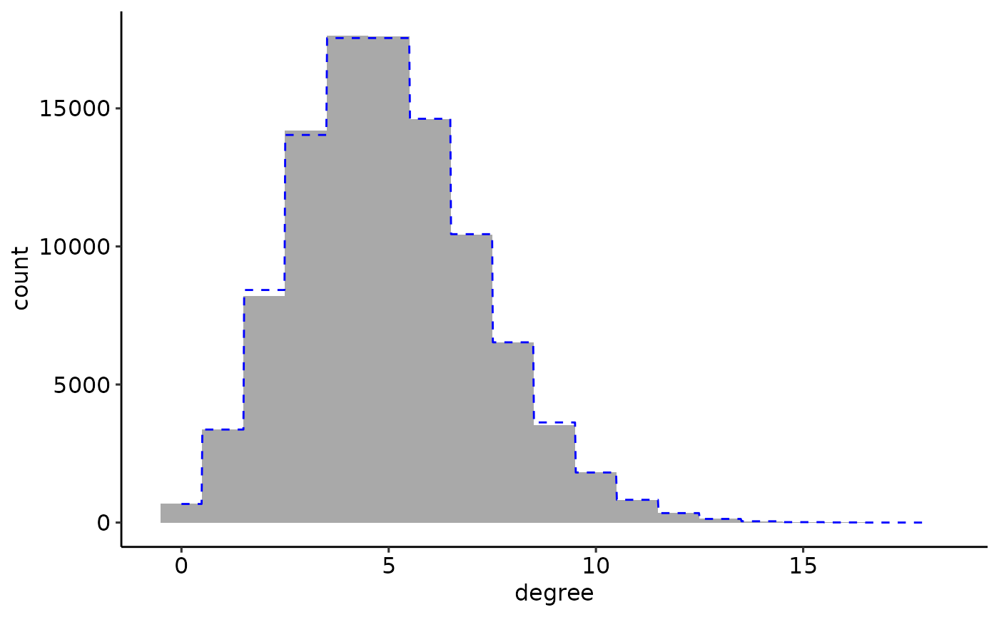

Creating and inspecting time distributions

Before we can start a simulation, we next have to create time distributions which represent the time it takes to transmit the disease across a link, and for the time it takes for an infected node to recover. We chose a log-normal distribution for the infection. By specifying p_infinity = 0.1, we modify the infection time distribution to produce an infinite infection time (i.e. no actual infection) in 10% of cases; this means that neighbours of an infected node only have a 90% chance of becoming infected eventually.

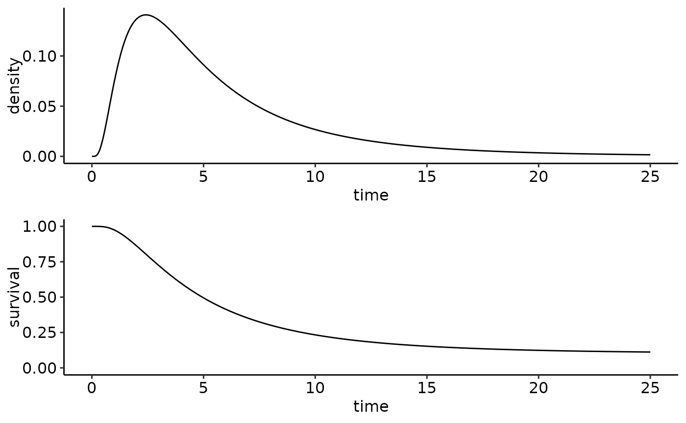
infection_time <- lognormal_time(mean=6, var=30, p_infinity = 0.1)

While time distribution objects are mainly useful for epidemic simulations, they can also be used similed to R’s built-in random distributions, see help(time_functions). We can, for example, plot the distribution’s density and survival function.

ggarrange(
  ggplot() +
    lims(x=c(0, 25)) + labs(x='time', y='density') +
    geom_function(fun=time_density, n=1000,
                  args=list(timedistribution=infection_time)),
  ggplot() +
    lims(x=c(0, 25), y=c(0,1)) + labs(x='time', y='survival') +
    geom_function(fun=time_survivalprobability, n=1000,
                  args=list(timedistribution=infection_time)),
  ncol=1
)

Creating and running simulations

To run a simulation, we now create a simulation object which binds together the network and the infection time distribution we created above

sim <- simulation(nw=nw, psi=infection_time)

Finally, we add an initial infection to get the epidemic going

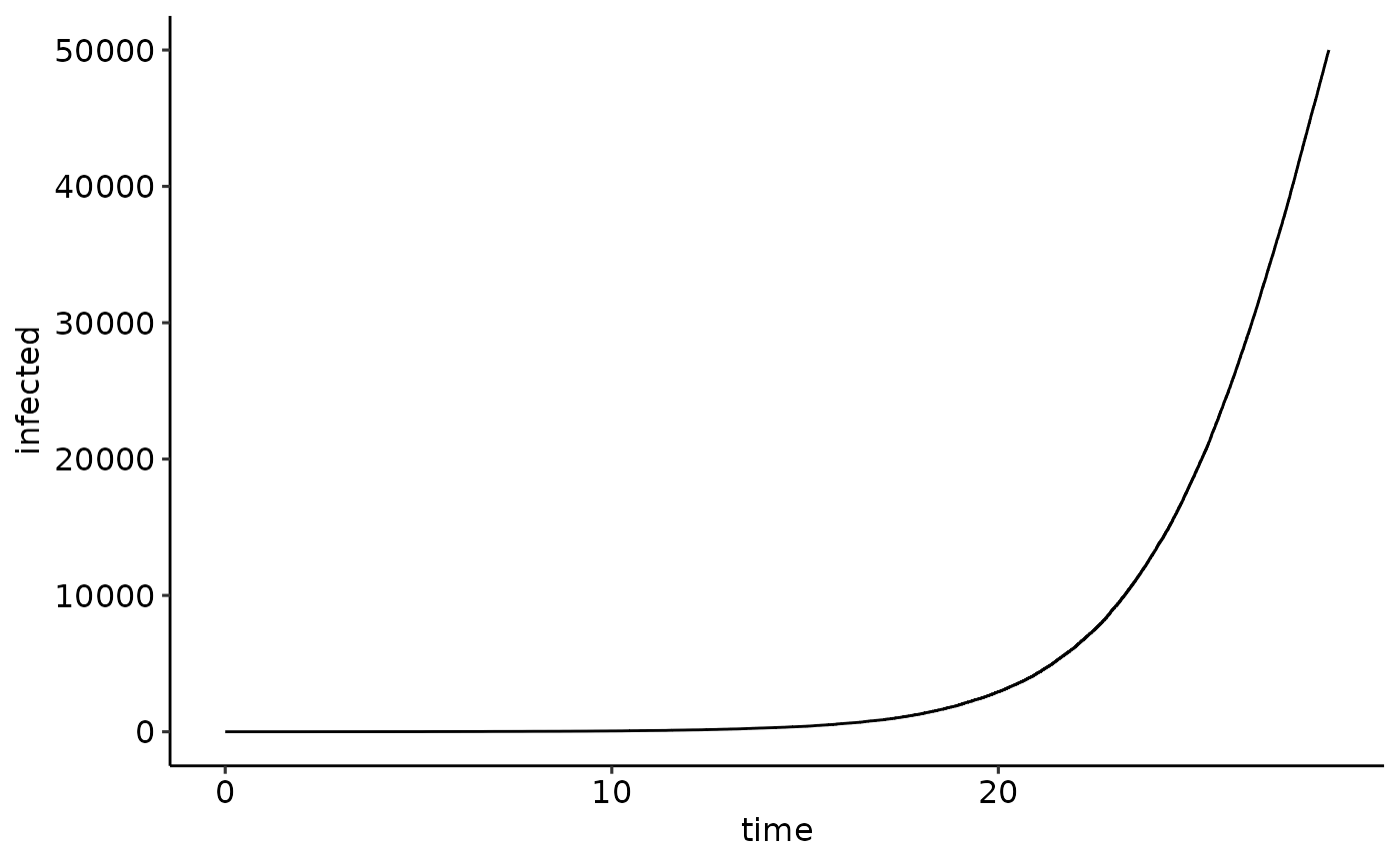
simulation_addinfections(sim, nodes=c(1), times=c(0.0))

and start the simulation, telling it to run until either time 100 or until 50,000 nodes have been infected.

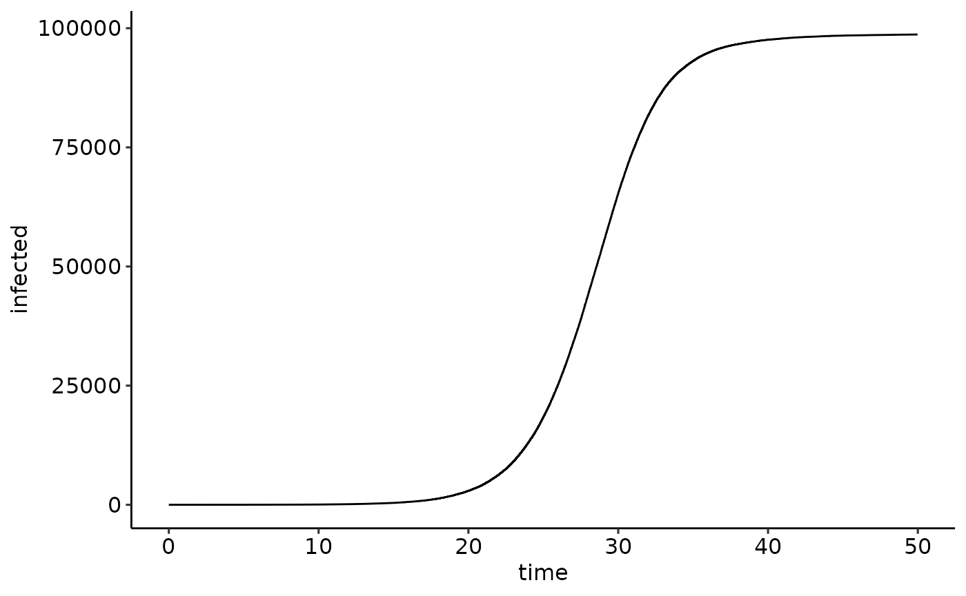
events <- simulation_run(sim, stop=list(time=100, total_infected=50e3))

Running a simulation returns a data.frame listing all the events that occurred. We can use this to plot the size of the epidemic over time.

ggplot(events) +
  geom_line(aes(x=time, y=infected))

Simulations can be continued by calling simulation_run again. To continue the simulation until time 50, we do

events2 <- simulation_run(sim, stop=list(time=50))

To plot the full trajectory, we must combine the events reported by the first call of simulation_run with the events reported by the second call,

ggplot(rbind(events, events2)) +
  geom_line(aes(x=time, y=infected))

Adding a recovery (or reset) time

In our previous simulation, nodes who were infected stayed infected indefinitely. We now add a recovery time so that nodes eventually return to their original state. Note that recovery here also implies that nodes become susceptible to reinfection; a better term may therefore be reset. For the recovery time distribution, we pick a weibull distribution

recovery_time <- weibull_time(shape=5, scale=50)
ggplot() +
  lims(x=c(0, 100)) + labs(x='time', y='density') +
  geom_function(fun=time_density,
                args=list(timedistribution=recovery_time))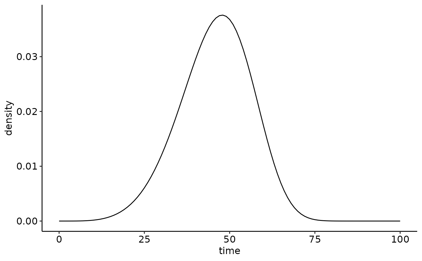

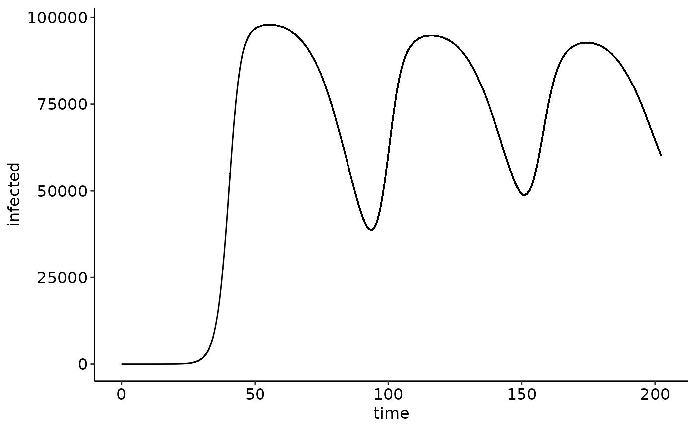
To run the simulation, we again create a simulation object, this time specifying the recovery time through the rho parameter. The trajectory now shows a wave-like pattern

sim <- simulation(nw=nw, psi=infection_time, rho=recovery_time)
simulation_addinfections(sim, nodes=c(1), times=c(0.0))
events <- simulation_run(sim, stop=list(time=300, total_infected=300e3))
ggplot(events) +
  geom_line(aes(x=time, y=infected))