Chapter 4. Reinforcement Learning#
Contents#
Bandit problem
Markov decision process (MDP)
Value functions
Dynamic programming (DP)
Q-learning and SARSA
Actor-Critic
Applications
Neural Mechanisms
Dopamine neurons
Basal ganglia
In reinforcement learning, an agent interacts with the environment by observing its state, sending an action, and receiving some reward.
Reinforcement learning in an agent-environment loop.
The aim of reinforcement learning is to find a policy, a mapping \(\pi\) from any state \(s\) to an action \(a\), that maximize the reward acquired.
a deterministic policy \(a=\pi(s)\)
a stochastic policy \(\pi(s,a)=p(a|s)\)
Bandit problem#
A simple case is that the state does not change, or change irrespective of the agent’s action. In this case, the problem is simply to estimate the expected reward for each action and pick the one with highest expected reward.
Markov decision process (MDP)#
A general setup for reinforcement learning is the Markov decision process (MDP), which is characterized by
finite state \(s \in S\)
finite actions \(a\in A(s)\)
state transition rule \(P(s'|s,a)\)
reward function \(R(s,a,s') = E[r|s,a,s']\)
There are two conventions for the time index of reward. The reward following \(a_t\) is denoted as \(r_t\) or \(r_{t+1}\) depending on the literature. Here we take the convention by Sutton and Barto (2018):
In a dynamical environment, an action at time \(t\) may affect the reward at later times \(r_\tau\), \(\tau > t\) through the state dynamics.
From the other viewpoint, a reward at time \(t\) may depend on all the past states and actions at \(\tau<t\).
Thus in selecting an action, an agent needs to consider maximizing expected cumulative reward, called return
finite horizon till time \(T\): \(R_t = r_{t+1} + r_{t+2} + ... + r_T\)
infinite horizon: \(R_t = r_{t+1} + \gamma r_{t+2} + \gamma^2 r_{t+3} + ...\)
where \(0\le\gamma<1\) is a discount factor to guarantee the sum to be finite.
Value Functions#
To evaluate the goodness of states, actions, and policy, a critical tool is the value function. There are two types.
State value function: expected return starting from a state \(s\) by following a policy \(\pi\)
(State-)Action value function: expected return by taking an action \(a\) at a state \(s\), and then following a policy \(\pi\)
An optimal policy \(\pi^*\) for and MDP is defined as a policy that satisfies
for any state \(s\in S\) and any policy \(\pi\).
The value functions for an optimal policy is called optimal value function and denoted as \(V^*(s)=V^{\pi^*}(s)\). An MDP can have multiple optimal policies, but the optimal value function is unique.
An optimal state value function and action value function are related by
Solving MDPs#
There are two main approaches in solving MDP problems
Model-based approach: Dynamic programming#
When the state transition function \(p(s'|s,a)\) and the reward function \(r(s,a)\) are known or learned:
Solve the Bellman equation for the optimal value function:
Use the optimal policy
Representative algorithms:
Policy iteration
Value iteration
Model-free approach: Reinforcement learning#
Do not assume that \(p(s'|s,a)\) and \(r(s,a)\) are unknown
Learn from the sequence of experience:
Representative algorithms:
SARSA
Q-learning
Actor-Critic
SARSA and Q Learning#
Estimate the action value function \(Q(s,a)\) using a table or ANN.
Select an action using the action value function
greedy: \(a = \arg\max_a Q(s,a)\)
\(\epsilon\)-greedy: random action with prob. \(\epsilon\) and greedy with prob. \(1-\epsilon\)
Boltzman:
\[p(a|s) = \frac{e^{\beta Q(s,a)}}{\sum_{b\in A}e^{\beta Q(s,b)}}\]Check the inconsistency of action value function estimates by the temporal difference (TD) error:
SARSA (on-policy):
Q learning (off-policy): assuming greedy policy from the next state
Update the action value function of the previous state and action in proportion to the TD error
import numpy as np
import matplotlib.pyplot as plt
%matplotlib inline
Classes for minimum environment and agent#
class Environment:
    """Class for a reinforcement learning environment"""

    def __init__(self, nstate=3, naction=2):
        """Create a new environment"""
        self.Ns = nstate   # number of states
        self.Na = naction  # number of actions

    def reset(self):
        """start an episode"""
        # randomly pick a state
        self.state = np.random.randint(self.Ns)
        return self.state

    def step(self, action):
        """step by an action"""
        # random reward
        self.reward = np.random.random()  # between 0 and 1
        # random next state
        self.state = np.random.randint(self.Ns)
        return self.state, self.reward
class Agent:
    """Class for a reinforcement learning agent"""

    def __init__(self, nstate, naction):
        """Create a new agent"""
        self.Ns = nstate   # number of states
        self.Na = naction  # number of actions

    def step(self, state, reward=None):
        """learn by reward and take an action"""
        # do nothing for reward
        # randomly pick an action
        self.action = np.random.randint(self.Na)
        return self.action
# Reinforcement non-learning
# Create the environment and the agent
env = Environment()
agent = Agent(env.Ns, env.Na)
# First contact
state = env.reset()
action = agent.step(state)
print([state, action])
# Repeat interactoin
for t in range(10):
    state, reward = env.step(action)
    action = agent.step(state, reward)
    print([t, reward, state, action])
[0, 0]
[0, 0.8017475463847797, 2, 0]
[1, 0.1704931340181257, 1, 0]
[2, 0.5749224924920653, 0, 1]
[3, 0.6370567378533448, 0, 1]
[4, 0.3097608767347664, 2, 1]
[5, 0.623897312376944, 2, 1]
[6, 0.08822929578107874, 0, 1]
[7, 0.7839652647127304, 2, 0]
[8, 0.1951692591005122, 2, 1]
[9, 0.5180369762116137, 2, 0]
class RL:
    """Reinforcement learning by interacton of Environment and Agent"""

    def __init__(self, environment, agent, nstate, naction):
        """Create the environment and the agent"""
        self.env = environment(nstate, naction)
        self.agent = agent(nstate, naction)

    def episode(self, tmax=50):
        """One episode"""
        # First contact
        state = self.env.reset()
        action = self.agent.step(state)
        # Table of t, r, s, a
        Trsa = np.zeros((tmax+1, 4))
        Trsa[0] = [0, 0, state, action]
        # Repeat interactoin
        for t in range(1, tmax+1):
            state, reward = self.env.step(action)
            action = self.agent.step(state, reward)
            Trsa[t,:] = [t, reward, state, action]
        return(Trsa)

    def run(self, nrun=10, tmax=50):
        """Multiple runs of episodes"""
        Return = np.zeros(nrun)
        for n in range(nrun):
            r = self.episode(tmax)[:,1]  # reward sequence
            Return[n] = sum(r)
        return(Return)
Example: Pain-Gain environment#
The Pain-Gain environment.
This is a Markov Decision Process that was designed for a functional MRI experiment (Tanaka et al. 2004). The environment has four states and two possible actions. By taking action 1, the state shift to the left and a positive reward is given, except at the leftmost state where it a big negative reward is given. By action 2, the state shift to the right and a negative reward is given, but at the rightmost state, a big positive reward is obtained. What is the right policy?
class PainGain(Environment):
    """Pain-Gain environment """

    def __init__(self, nstate=4, naction=2, gain=6):
        super().__init__(nstate, naction)
        # setup the reward function as an array
        self.R = np.ones((self.Ns, self.Na)) # small gains
        self.R[:,1] = -1   # small pains for 2nd action (a=1)
        self.R[0,0] = -gain  # large pain
        self.R[-1,1] = gain  # large gain

    def step(self, action):
        """step by an action"""
        # reward by the reward matrix
        self.reward = self.R[self.state, action]
        # move left or right and circle
        self.state = (self.state + 2*action-1)%self.Ns
        return self.state, self.reward
class QL(Agent):
    """Class for a Q-learning agent"""

    def __init__(self, nstate, naction):
        super().__init__(nstate, naction)
        # allocate Q table
        self.Q = np.zeros((nstate, naction))
        # default parameters
        self.alpha = 0.1  # learning rate
        self.beta = 1.0   # inverse temperature
        self.gamma = 0.9  # discount factor

    def boltzmann(self, q):
        """Boltzmann selection"""
        pr = np.exp( self.beta*q)   # unnormalized probability
        pr = pr/sum(pr)    # probability
        return np.random.choice(len(pr), p=pr)

    def step(self, state, reward=None):
        """learn by reward and take an action"""
        if reward != None:
            # TD error: self.state/action retains the previous ones
            delta = reward + self.gamma*max(self.Q[state,:]) - self.Q[self.state,self.action]
            # Update the value for previous state and action
            self.Q[self.state,self.action] += self.alpha*delta
        # Boltzmann action selection
        self.action = self.boltzmann( self.Q[state,:])
        # remember the state
        self.state = state
        return self.action
# Pain-Gain environment and Q-learning agent
pgq = RL(PainGain, QL, 4, 2)
# customize parameters
pgq.agent.beta = 2
# run an episode
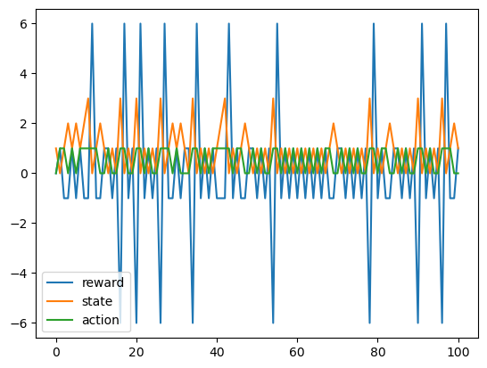
trsa = pgq.episode(100)
plt.plot(trsa[:,1:]);
plt.legend(("reward", "state", "action"));
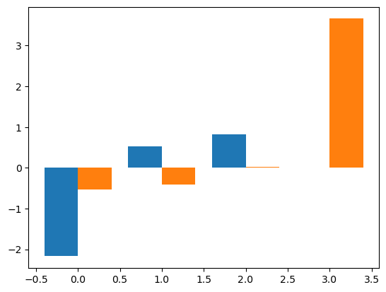
# Visualize Q function
plt.bar(np.arange(4)-0.2, pgq.agent.Q[:,0], 0.4 )  # action0
plt.bar(np.arange(4)+0.2, pgq.agent.Q[:,1], 0.4 );  # action1
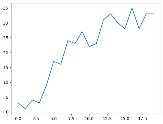
# Repeat episodes for learning curve
pgq = RL(PainGain, QL, 4, 2)
R = pgq.run(20, 50)
plt.plot(R);
Actor-Critic#
Another popular class of RL is Actor-Critic.
Actor implements a policy \(\pi_\w=p(a|s;\w)\), where \(\w\) is the parameter, such as the elements of a table or the weights of an ANN.
Critic learns the state value function of the actor’s policy \(\pi_\w\):
using a table or an ANN.
Learning is based on the temporal difference (TD) error:
The TD error is used for learning of both critic and actor, but in different ways:
Critic:
Actor:
or
Dopamine neurons#
Dopamine neurons in the midbrain appear to code TD error (Schultz et al. 1997).
Basal ganglia#
A reinforcement learning model of the basal ganglia (Doya 2007).
References#
Sutton RS, Barto AG (2018). Reinforcement Learning: An Introduction, 2nd edition. MIT Press.
(http://incompleteideas.net/book/the-book-2nd.html)Barto AG, Sutton RS, Andersen CW (1983). Neuronlike adaptive elements that can solve difficult learning control problems. IEEE Transactions on Systems, Man, and Cybernetics, 13, 834-846. http://doi.org/10.1109/TSMC.1983.6313077
Doya K (2007). Reinforcement learning: Computational theory and biological mechanisms. HFSP J, 1, 30-40. http://doi.org/10.2976/1.2732246/10.2976/1
Dopamine neurons#
Schultz W, Dayan P, Montague PR (1997). A Neural Substrate of Prediction and Reward. Science, 275, 1593-1599. http://doi.org/10.1126/science.275.5306.1593
Nomoto K, Schultz W, Watanabe T, Sakagami M (2010). Temporally extended dopamine responses to perceptually demanding reward-predictive stimuli. J Neurosci, 30, 10692-702. http://doi.org/10.1523/JNEUROSCI.4828-09.2010
Basal ganglia#
Samejima K, Ueda Y, Doya K, Kimura M (2005). Representation of action-specific reward values in the striatum. Science, 310, 1337-40. http://doi.org/10.1126/science.1115270
Ito M, Doya K (2015). Distinct neural representation in the dorsolateral, dorsomedial, and ventral parts of the striatum during fixed- and free-choice tasks. Journal of Neuroscience, 35, 3499-3514. http://doi.org/10.1523/JNEUROSCI.1962-14.2015