Chatper 6. Bayesian Approaches

Chatper 6. Bayesian Approaches#

\[ % Latex macros \newcommand{\mat}[1]{\begin{pmatrix} #1 \end{pmatrix}} \newcommand{\p}[2]{\frac{\partial #1}{\partial #2}} \renewcommand{\b}[1]{\boldsymbol{#1}} \newcommand{\c}[1]{\mathcal{#1}} \]

Contents#

Bayes’ theorem
Bayesian linear regression (Bishop, Chater 3)
Bayesian model comparison
Bayesian networks (Bishop, Chater 8)
Dynamic Bayesian inference
Bayesian Brain
- Sensory psychophysics
- Cortical circuit

Bayes’ Theorem#

From the product rule of the joint probability

\[ p(X,Y) = p(Y|X) p(X) \]

and the symmetry of joint probability

\[ p(X,Y)=p(Y,X),\]

we have the relationship

\[ p(X|Y)p(Y) = p(Y|X)p(X),\]

which brings us to Bayes’ theorem:

\[ p(X|Y) = \frac{p(Y|X)p(X)}{p(Y)}. \]

Bayes’ theorem relates a conditional probability $p(X|Y)$ to the one in the opposite direction $p(Y|X)$. This simple formula, however, has turned out to be very insightful in the context of sensory processing and learning.

Suppose $X$ is an invisible state of your interest, such as a prey or predator hiding in a bush, and $Y$ is a noisey sensory observation.

Your knowledge or assumption about the state probability of different states is represented by $p(X)$, called prior probability.
What sensory input $Y=y$ is observed if the state is $X=x$ is represented by a sensory observation model $p(Y|X)$.
For a given sensory observation $y$, the probability for such an observation with the state $x$ $p(Y=y|X=x)$ is as the likelihood of the state $x$. As a function of differnt states $X$, $p(Y=y|X)$ is called the likelihood function.
The probability of the state $X$ after observing $y$, $p(X|Y=y)$ is called the posterior probability.

Bayes’ theorem in this case

\[ p(X|Y=y) = \frac{p(Y=y|X)p(X)}{p(Y=y)} \]

\[ \propto p(Y=y|X)p(X) \]

gives a theoretical basis of how to combine the prior knowledge $p(X)$ and sensory evidence $y$.
It is intuitive that the posterior probability $p(X|Y=y)$ is proportional to the product of the prior prbability $p(X)$ and the likelihood $p(Y=y|X)$ for oberving $y$.

The denominator $p(Y=y)$ is called the marginal likelhood and serves as the normalizing factor so that the posterior probability sums or intergrates to one.

The marginal likelhood $p(Y=y)$ is the probability of observing $y$ by considering all the possible states $X$, and generally computed by marginalizing the joint probability

\[ p(Y=y) = \sum_X p(Y=y|X=x)p(X=x) \]

or

\[ p(Y=y) = \int_X p(Y=y|X=x)p(X=x) dx. \]

Example: mouse in a bush#

You are a cat chasing a mouse and saw it ran behind three bushes.

You know about half of the case a hiding mouse makes a sound, but about 10% of the time you hear sound just by the wind. That gives you a sensory observation model:

$p(Y \vert X)$	no mouse $X=0$	mouse hiding $X=1$
no sound $Y=0$	0.9	0.5
sound $Y=1$	0.1	0.5

Then you heard a rustuling sound from one bush. Then what is the probability of a mouse hiding behind the bush, $p(X=1|Y=1)$? From the above table, 0.5?

No, actually. In the ‘heard’ row, 0.1 and 0.5 do not sum up to one. They are likelihoods $p(Y=1|X)$, but not probability distribution $p(X|Y=1)$ for the mouse to be in the bush or not.

The mouse should be one of the three bushes, so you would assume that the prior probability of the mouse in this bush is 1/3:

prior probability	no mouse $X=0$	mouse hiding $X=1$
$p(X)$	2/3	1/3

By having this prior probability, we can use Bayes’ theorem:

\[ p(X=1|Y=1) = \frac{p(Y=1|X=1)p(X=1)}{p(Y=1|X=0)p(X=0)+p(Y=1|X=1)p(X=1)} \]

\[ = \frac{0.5*1/3}{0.1*2/3+0.5*1/3} = \frac{5}{7} \simeq 0.71 \]

Iterative Bayesian Inference#

A useful property of Bayesian inference is that you can apply it iteratively to incoming data stream.

We denote the sequence of observations up to time $t$ as

\[ y_{1:t}=(y_1,...,y_t) \]

and want to estimate the cause $x$ of these observations

\[ p(x|y_{1:t}) = \frac{p(y_{1:t}|x)\ p(x)}{p(y_{1:t})} \]

If the observations are independent, their joint distribution is a product

\[ p(y_{1:t}|x) = p(y_1|x)\cdots p(y_t|x) \]

and thus the posterior can be decomposed as

\[ p(x|y_{1:t}) = \frac{p(y_1|x)\cdots p(y_{t-1}|x)\ p(y_t|x)\ p(x)}{p(y_1)\cdots p(y_{t-1})\ p(y_t)} \]

\[ = \frac{p(y_t|x)}{p(y_t)}\ \frac{p(y_1|x)\cdots p(y_{t-1}|x)\ p(x)}{p(y_1)\cdots p(y_{t-1}) } \]

\[ = \frac{p(y_t|x)\ p(x|y_{1:t-1})}{p(y_t)}. \]

This means that the posterior $p(x|y_{1:t-1})$ that you computed by time $t-1$ serves as the prior to be combined with the likelihood for the new coming data $p(y_t|x)$ for computing the new posterior $p(x|y_{1:t})$.

This iterative update of the posterior is practically helpful in online inference utilizing whatever data available so far.

Coin toss#

Here is a simple example of estimating the parameter $\mu$, probability for a coin to land head up, during multiple tosses.

import numpy as np
import scipy.stats
import matplotlib.pyplot as plt
%matplotlib inline

# take samples
mu = 0.4  # probability of head
N = 10   # number of samples
y = np.random.choice(2, N, p=[1-mu, mu]) # binary observation sequence
y

array([0, 1, 0, 1, 0, 0, 0, 0, 0, 1])

dx = 0.01  # plot step
x = np.arange( 0, 1, dx)  # range of the parameter
prior = np.ones( len(x))  # Assume a uniform prior
plt.figure(figsize=(6,10))
for t in range(N):
    plt.subplot(N//2, 2, t+1)  # a new figure
    # prior
    plt.plot( x, prior, 'b')
    # observation
    plt.plot( y[0:t+1], np.arange(t+1)/N, 'ko')
    # likelihood
    likelihood = x*y[t] + (1-x)*(1-y[t]) # theta if head, 1-theta if tail
    plt.plot( x, likelihood, 'g')
    # product
    prilik = prior*likelihood
    plt.plot( x, prilik,'c')
    # posterior by normalization
    marginal = sum(prilik)*dx    # integrate over the parameter range
    posterior = prilik/marginal  # normalize
    plt.plot( x, posterior, 'r')
    plt.xlabel(r'$\mu$')
    if t==0:
        plt.legend(('prior', 'observation', 'likelihood', 'prior*like.', 'posterior'))
    plt.title(f't = {t+1}')
    # posterior as a new prior
    prior = posterior
plt.tight_layout()

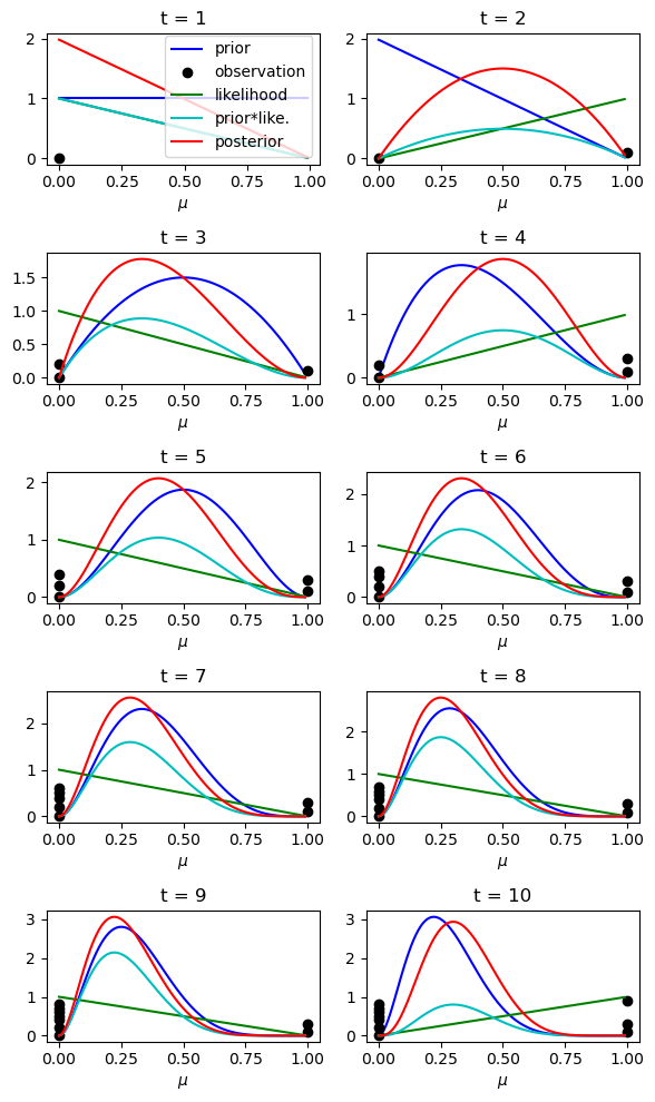
_images/ec298bd40eef7e8cf7715a33ee2911d3901870cadaa1178f7a68b4e38801e660.png

As more data are collected, the posterior distribution of $\mu$ becomes sharper and colser to the true value.

For binary observations $y_{1:n}=(y_1,...,y_n)$, under uniform prior probability, the posterior probability of the mean $mu$ is

\[ p(\mu|y_{1:n}) \propto \mu^{n_1} (1-\mu)^{n_0} \]

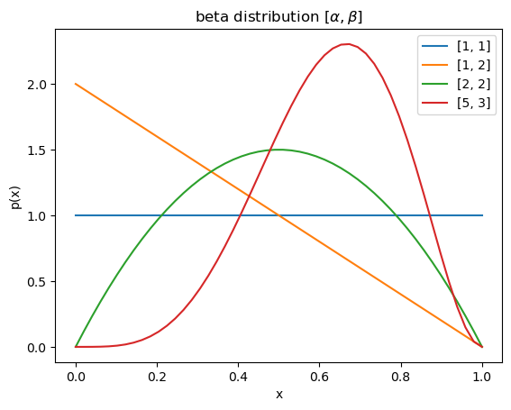
where $n_1$ and $n_0$ are the number of observations of $1$ and $0$, respectively. This is an example of beta distribution:

\[ p(x; \alpha, \beta) \propto x^{\alpha-1} (1-x)^{\beta-1} \]

with $\alpha=n_1+1$ and $\beta=n_0+1$. A uniform prior distribution is represented by $\alpha = \beta = 1$.

If a prior and the posterior are represented by the same class of distribution, the prior is called the conjugate prior for the observation model. Beta distribution is the conjugate prior for the binary (Bernoulli) observation.

alpha_beta = [[1,1], [1,2], [2,2], [5,3]]
x = np.linspace(0., 1.)
for ab in alpha_beta:
    p = scipy.stats.beta.pdf(x, ab[0], ab[1])
    plt.plot(x, p)
plt.xlabel('x'); plt.ylabel('p(x)')
plt.title(r'beta distribution $[\alpha,\beta]$')
plt.legend(alpha_beta);

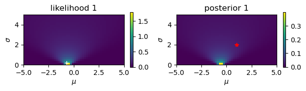
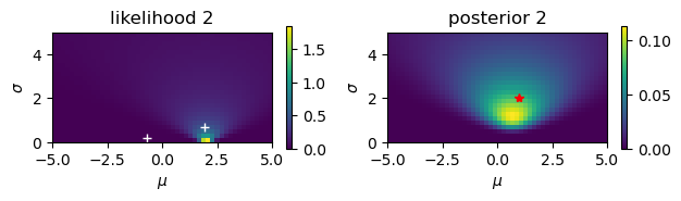
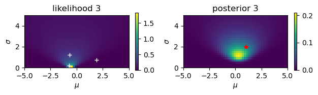
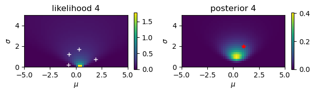
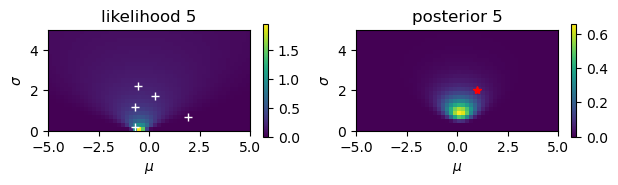
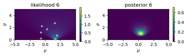
_images/59e2e5ae80fbc8dc51b66e81a3f85fcbd06e40dbc8ad4de9bcfeb4e79f9176a3.png

Gaussian observations#

Estimate the mean $\mu$ and the standard deviationn $\sigma$ from noisy observations.

# Noisy observation: y = N(mu,sigma)
mu = 1
sigma = 2
N = 10
y = mu + sigma*np.random.randn(N)
print(y)

[-0.70635196  1.92218514 -0.68584733  0.2965167  -0.55829412  1.58621975
 -0.26925025  2.82542414  2.778251    1.31513282]

# Start from a uniform prior
rmu = 5; dmu = 0.2   # range and step of mu
rsig = 5;  dsig = 0.2 # range and step of sigma
m = np.arange(-rmu, rmu, dmu)
s = np.arange(rsig, 0, -dsig)
M, S = np.meshgrid(m, s)  # grid of mu and sigma
prior = np.ones_like(M)/(2*rmu*rsig)

for n in range(N):
    plt.figure()
    plt.subplot(1, 2, 1)
    # observation
    plt.plot( y[0:n+1], dsig+rsig*np.arange(n+1)/N, 'w+')
    # likelihood
    likelihood = np.exp(-((y[n]-M)/S)**2/2)/(np.sqrt(2*np.pi)*S)
    plt.imshow(likelihood, extent=(-rmu,rmu,0,rsig))
    plt.xlabel(r'$\mu$'); plt.ylabel(r'$\sigma$');
    plt.title(f'likelihood {n+1}')
    plt.colorbar(shrink=0.25)
    # posterior
    plt.subplot(1, 2, 2)
    prilik = prior*likelihood
    #plt.imshow(prilik, extent=(-rmu,rmu,0,rsig))
    marginal = np.sum(prilik)*dmu*dsig
    posterior = prilik/marginal
    plt.imshow(posterior, extent=(-rmu,rmu,0,rsig))
    plt.xlabel(r'$\mu$'); plt.ylabel(r'$\sigma$');
    plt.title(f'posterior {n+1}')
    prior = posterior  # new prior
    plt.colorbar(shrink=0.25)
    # true value
    plt.plot( [mu], [sigma], 'r*')
    plt.tight_layout()

_images/a6cb7ec8e83788f93f4c3799a8ae8a156f08ed0b4a255207a49c5ac6baf68532.png

_images/11392f3d8c77ac5521fea5dfe13b1e933db2c974cbd607ae9aacdab489bd3f0d.png

_images/881b815788f5e2c39979f5f735da18eb31b6e78328945b2231ce0eca8be57a9a.png

_images/ae1456610f5374542e859f794b91578c16ea1434c6fca2cac2a3366fb1262f14.png

_images/c9d18440aa79299f7d481657822ebfbb8e78883833a02bc74ed1e19423fc66fe.png

_images/c3215f7c0293c616408f0e2c2ba23a6e941bebd8c4c3c5710e4649b6d0e0e130.png

_images/a4d558815c6b2f026e0434a250b94355fe39af5a56873c2aaeafc6997ff3ff39.png

_images/9872bf0925a6dc98b456d00c260b122f5893decef5fa762ae4a6c405c95ea101.png

_images/3b8edba20fe838c236bc8c16eeeaf5f8a169e2d6d353bd6d9149cfae955cddd8.png

_images/47369dd58c832f6fb2ee4e97d0eed7f86c4bfe1a1162f17a9cc75105c58809ec.png

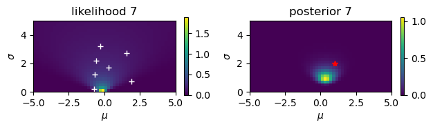
Here we consider a case where $y$ is an observation of $x$ with Gaussian noise

\[ p(y|x) \propto e^{-\frac{(y-x)^2}{2\sigma_1^2}} \]

If we assume that the prior distribution of $x$ is also Gaussian

\[ p(x) \propto e^{-\frac{(x-\mu_0)^2}{2\sigma_0^2}} \]

then the posterior distribution also takes a Gaussian form:

\[ p(x|y) \propto p(x)p(y|x) \propto e^{-\frac{(x-\mu_0)^2}{2\sigma_0^2}} e^{-\frac{(y-x))^2}{2\sigma_1(x)^2}} = e^{-\frac{(x-\mu_0)^2}{2\sigma_0^2} - \frac{(x-y)^2}{2\sigma_1^2}} \propto e^{-\frac{(x-\mu_2)^2}{2\sigma_2^2}} \]

By considering the coefficients of $x^2$ and $x$ of the exponent, we have

\[ \frac{1}{\sigma_0^2}+\frac{1}{\sigma_1^2} = \frac{1}{\sigma_2^2} \]

\[ \frac{\mu_0}{\sigma_0^2}+\frac{y}{\sigma_1^2} = \frac{\mu_2}{\sigma_2^2} \]

From these we find the mean and the variance of the posterior as

\[ \sigma_2^2 = \frac{1}{\frac{1}{\sigma_0^2}+\frac{1}{\sigma_1^2}} = \frac{\sigma_0^2 \sigma_1^2}{\sigma_0^2+\sigma_1^2} \]

\[ \mu_2 = \frac{\sigma_2^2}{\sigma_0^2}\mu_0+\frac{\sigma_2^2}{\sigma_1^2}y = \frac{\sigma_1^2}{\sigma_0^2+\sigma_1^2}\mu_0+\frac{\sigma_0^2}{\sigma_0^2+\sigma_1^2}y \]

The mean of the posterior is a weighted average of the mean of the prior and the new observation; larger the weight for smaller the variance.

If there are multiple independent observations, such as by vision, audition, and haptics, they should also be weighting based on the ratio of the variances of sensory obervations.

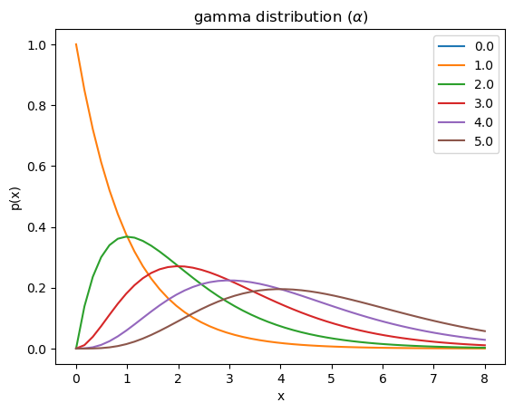
For a Gaussian likelihood function, the conjugate priors for the mean $\mu$ is also a Gaussian. As we saw many $\frac{1}{\sigma^2}$ above, it is often more convenient to parameterize a Gaussian distribution by the inverse variance, or the precision $\lambda=\frac{1}{\sigma^2}$. For the presicision, the conjugate prior is a Gamma distribution

\[ p(\lambda) \propto \lambda^{\alpha-1}e^{-\lambda}. \]

alpha = np.arange(6.)
x = np.linspace(0., 8.)
for a in alpha:
    p = scipy.stats.gamma.pdf(x, a)
    plt.plot(x, p)
plt.xlabel('x'); plt.ylabel('p(x)')
plt.title(r'gamma distribution $(\alpha)$')
plt.legend(alpha);

_images/5a1ae1d00f0b6812206b885ed18114a15b0e0d12c1e775fd39319f1e7dcb99eb.png

Bayesian approaches in machine learning#

“Bayesian” is quite popular in machine learning, but it is used for different meanings:

To combine prior knowledge and the likelihood from observation
To assume a graphical model of data generation for estimation of the causes
To estimate the distribution of a variable, not a single point

In supervised learning:

avoid over fitting by introducing a prior distribution on the parameters
compare models by their probability of producing observed data

In reinforcement learning:

infer the environmental state from incomplete observation
estimate the distribution of reward, not just the expectation

In unsupervised learning:

infer hidden variables behind data
- e.g. responsibility in Mixtures of Gaussians

Bayesian Linear Regression#

The standard linear regression (Chapter 3) assumes a linear regression function with additive noise $$ t_n = \b{w}^T\b{x}_n + \epsilon $$ where $p(\epsilon)=\mathcal{N}(0,\beta^{-1})$.

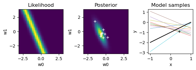
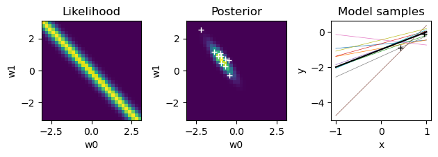
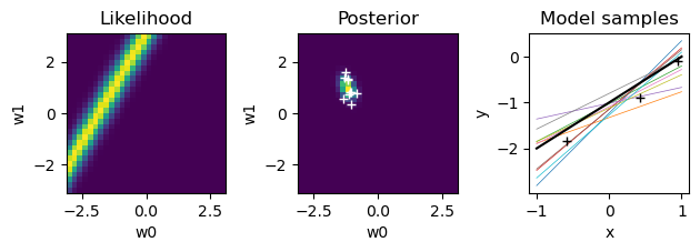
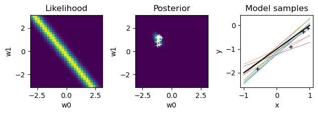
In Bayesian linear regression, we assume that the weights are sampled from a prior distribution $p(\b{w})=\mathcal{N}(\b{0},\alpha^{-1}I)$.

The likelihood of the parameter $\b{w}$ for the target output $\b{t}$ is

\[ p(\b{t}|X, \b{w}, \beta) = \prod_{n=1}^N \mathcal{N}(t_n|\b{w}^T\b{x}_n,\beta^{-1}) \]

When both the prior and likelihood are Gaussian, the posterior will also be Gaussian and have the form:

\[ p(\b{w}|\b{t}) = \mathcal{N}(\b{w}|\b{m},S) \]

where the mean of the posterior weights is given as

\[ \b{m} = \beta S X^T \bf{t} \]

and the variance as

\[ S = (\alpha I + \beta X^T X)^{-1} \]

If we let $\alpha=0$, i.e. infinitely large variance for the weight prior, this is equivalent to regular linear regression.

The log posterior probability of weights is given by

\[ \log p(\b{w}|\b{t}) = - \frac{\beta}{2}\sum_{n=1}^N \{t_n - \b{w}^T \b{x}_n\}^2 - \frac{\alpha}{2} \b{w}^T\b{w} +\mbox{const.}\]

This presents a link with a common method of adding a penalty term for the size of the weights, or equivallently adding diagonal component in the data correlation matrix, know as ridge regression, which minimizes

\[ E(\b{w}) = \frac{1}{2}\sum_{n=1}^N \{t_n - \b{w}^T \b{x}_n\}^2 + \frac{\lambda}{2} \b{w}^T\b{w} \]

The Bayesian regression gives a probabilistic interpretation of the regularization parameter as $\lambda=\frac{\alpha}{\beta}$.

# We will use this frequently
def gauss(x, mu=0, sigma=1):
    """Gaussian distribution"""
    return np.exp(-((x-mu)/sigma)**2/2)/(np.sqrt(2*np.pi)*sigma)

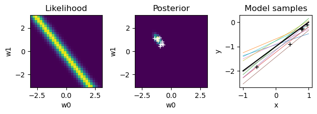
# Distributions in the parameter and data spaces
alpha = 1.  # inverse variance of weight prior
beta = 10  # inverse variance of observation noise
wt = np.array([-1, 1])  # 'true' weights
# sample data
N = 6
xrange = [-1, 1]
X = np.random.uniform(xrange[0], xrange[1], size=N)
X = np.c_[np.ones(N), X]  # prepend 1 in the leftmost column
t = wt@X.T + np.random.normal(size=N)/np.sqrt(beta)  # targets with noise
# for weight space visualization
W = np.linspace(-3, 3, 30)
W0, W1 = np.meshgrid(W, W)
K = 10  # weight samples
pw = gauss(W0)*gauss(W1)
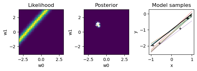
for n in range(N):
    plt.figure()
    # likelihood
    like = gauss(t[n] - (W0+W1*X[n,1]), sigma=beta**(-0.5))
    plt.subplot(1,3,1)   # left
    plt.pcolormesh(W, W, like)
    plt.axis('square')
    plt.title("Likelihood"); plt.xlabel("w0"); plt.ylabel("w1");
    # new posterior
    S = np.linalg.inv(alpha*np.eye(2) + beta*X[:n+1].T@X[:n+1])
    m = beta*S@X[:n+1].T@t[:n+1]
    # print(n, ': m =', m, '; S =', S)
    plt.subplot(1,3,2)
    post = pw*like
    plt.pcolormesh(W, W, post)
    plt.axis('square')
    plt.title("Posterior"); plt.xlabel("w0"); plt.ylabel("w1");
    # sample weights
    wpost = np.random.multivariate_normal(m, S, K)
    plt.plot(wpost[:,0], wpost[:,1], "w+")
    # plot model samples
    xrange = np.array([-1., 1.])   # range of input x
    plt.subplot(1,3,3)
    for k in range(K):
        plt.plot(xrange, wpost[k,0]+wpost[k,1]*xrange, lw=0.5)
    # true line
    plt.plot(xrange, wt[0]+wt[1]*xrange, "k")
    plt.plot(X[:n+1,1], t[:n+1], "k+")  # training data
    plt.gca().set_box_aspect(1)
    plt.title("Model samples"); plt.xlabel("x"); plt.ylabel("y");
    plt.tight_layout()  # adjust subplot margins
    pw = post

_images/cd8c868669cb5703042c183777b39849dad456abbd3966aa98546750437e41d8.png

_images/d83917b153309daf1d27c59a028312eb01fb3ffeaef939ed56c50e57925df9f4.png

_images/1f52fdfb52a3dc60c36c2490185ce6de72bf0d8ee763596af0e84d7d1cdae747.png

_images/0b0daec5fc3b59edb060c6a47fada88d7d31555da9898038ba0926be4c7783e7.png

_images/0befbe3a34c800531f217093fa93ad647827667e85e090fa88fe16c0e156fe2f.png

_images/5c19a5e7e1d394810c3655f4376468ece2f8bf9b375b7cd25cc4b38b0e3c3dc8.png

Predictive distribution#

In Bayesian regression, the result is not one weight vector, but a distribution in the weight space. Then it is reasonable to consider the distribution of the output considering such uncertainty in the weigts.

The output $y$ for a new input $\b{x}$ should have the distribution

\[ p(y|\b{x},\b{t},\alpha,\beta) = \int p(y|\b{x},\b{w},\beta) p(\b{w}|\b{t},\alpha,\beta) d\b{w} \]

\[ = \mathcal{N}(t|\b{m}^T \b{x}, \sigma^2(\b{x})) \]

where the variance of the output is given by

\[ \sigma^2(\b{x}) = \beta^{-1} + \b{x}^T S \b{x} \]

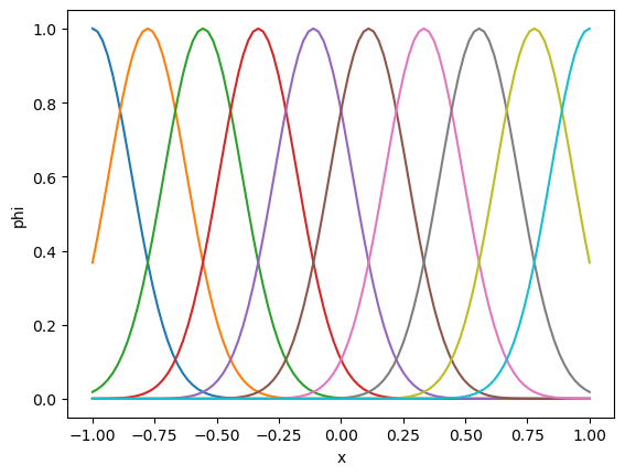
Let us see the example of approximating a sine function by Gaussian basis functions.

# 1D Gaussian basis functions 
def gbf1(x, xrange=[-1.,1.], M=10):
    """Gaussian basis functions: x can be a 1D array"""
    xc = np.linspace(xrange[0], xrange[1], num=M)  # centers
    xd = (xc[1]-xc[0])  # interval
    # x can be an array for N data points
    return np.exp(-((np.tile(x,[M,1]).T - xc)/xd)**2)
# example
x = np.linspace(-1, 1, 100)
plt.plot(x, gbf1(x, M=10));
plt.xlabel("x"); plt.ylabel("phi");

_images/6502caeed6c5b16f748e795ba9f301cc7fc8619a4f7b1b1191eace8947dedaf9.png

def blr(X, t, alpha=1., beta=10.):
    """Bayesian linear regression
    alpha: inv. variance of weight prior 
    beta: inv. variance of observation noise
    """
    N, D = X.shape
    S = np.linalg.inv(alpha*np.eye(D) + beta*X.T@X) # posterior covariance
    m = beta*S@X.T@t   # posterior mean
    return m, S

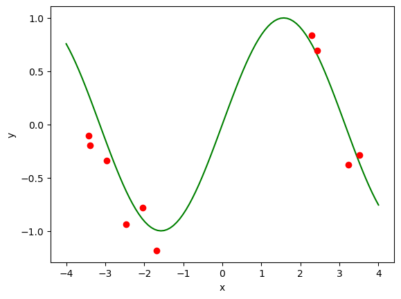
def target(x):
    """Target function"""
    return np.sin(x)

# Training data
N = 10
eps = 0.2  # noise size
xr = 4   # range of x
x = np.random.uniform(-xr, xr, size=N)  
f = target(x)  # target function
t = f + np.random.normal(scale=eps, size=N) # with noise
# data for testing/plotting
Np = 100
xp = np.linspace(-xr, xr, Np)
fp = target(xp)
plt.plot(xp, fp, "g")  # target function
plt.plot(x, t, "ro");  # training data
plt.xlabel("x"); plt.ylabel("y");

_images/72e3a772f5ccb3efa79b2fe0af58e844507a13890da66ac618f21edc5438dbba.png

M = 10  # number of basis functions
Phi = gbf1(x, [-xr,xr], M)  # Gaussian basis functions
m, S = blr(Phi, t, alpha=1., beta=10)  # Bayesian linear regression
print(m)
# test data
Phip = gbf1(xp, [-xr,xr], M)
yp = Phip@m.T
plt.plot(xp, fp, "g")  # target function
plt.plot(x, t, "ro");  # training data
plt.plot(xp, yp, "b");  # MAP estimate
# predictive distribution
sigma = np.sqrt(1/beta + np.sum(Phip@S*Phip, axis=1))
plt.plot(xp, yp+sigma, "c")
plt.plot(xp, yp-sigma, "c")
plt.xlabel("x"); plt.ylabel("y");

[ 0.08160849 -0.10824807 -0.61026033 -0.66746323 -0.15525576  0.00855041
  0.31424315  0.83447899 -0.36854145 -0.20883743]

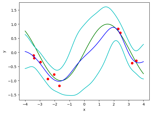
_images/9e1ac50e3a8f16347aa8633f7999f858dd345920f260ec9234a99fe0a9f43495.png

See how $N$, $M$, $\alpha$ and $\beta$ affect the performance.

Bayesian model comparison#

We have so far considered Bayesian inference of the parameter $\b{w}$ for a given model $\c{M}$, such as a regression model with some input variables, but we can also think of Bayesian inference of probability over models $\c{M}_i$, such as regression models with different choices of input variables, given data $\c{D}$

\[ p(\c{M}_i|\c{D}) \propto p(\c{M}_i) p(\c{D}|\c{M}_i). \]

Here $p(\c{D}|\c{M}_i)$, the likelihood of a model given data, is called the evidence of the model.

If we include a model explicitly in our Bayesian parameter estimation, we have

\[ p(\b{w}|\c{D},\c{M}_i) = \frac{p(\c{D}|\b{w},\c{M}_i)p(\b{w}|\c{M}_i)}{p(\c{D}|\c{M}_i)}, \]

where we have the evidence as the normalizing denominator

\[ p(\c{D}|\c{M}_i) = \int p(\c{D}|\b{w},\c{M}_i)p(\b{w}|\c{M}_i) d\b{w}. \]

This is also called marginal likelihood because it is the likelihood of the model with its parameters marginalized.

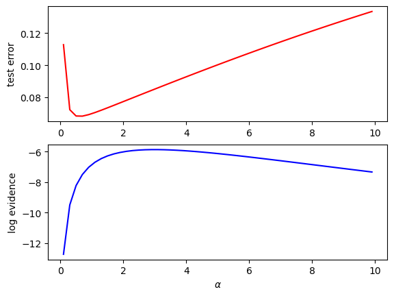
Computing model evidence#

In Bayesian linear regression, the model evidence with the hyperparamters $\alpha$ (weight prior) and $\beta$ (observation noise) is given by integration over all the range of the weight parameters $\b{w}$:

\[ p(\b{t}|\alpha,\beta) = \int p(\b{t}|\b{w},\beta)p(\b{w}|\alpha) d\b{w}, \]

The log evidence is given as (Bishop, Chapter 3.5)

\[ \log p(\b{t}|\alpha,\beta) = -\frac{\beta}{2} ||\b{t}-X\b{m}||^2 - \frac{\alpha}{2} ||\b{m}||^2 \]

\[ + \frac{1}{2}\log|S| + \frac{D}{2}\log\alpha + \frac{N}{2}(\log\beta - \log(2\pi)) \]

where $\b{m}$ and $S$ also depend on $\alpha$ and $\beta$.

def logev(X, t, m, S, alpha, beta):
    """log evidence for Bayesian regression
    m: posterior mean
    S: posterior covariance
    alpha: inv. variance of weight prior 
    beta: inv. variance of observation noise
    """
    N, D = X.shape
    #S = np.linalg.inv(alpha*np.eye(D) + beta*X.T@X) # posterior covariance
    #m = beta*S@X.T@t   # posterior mean
    em = t - X@m.T  # error with MAP estimate
    #alpha = D/np.dot(m,m)
    #beta = N/np.dot(em,em)
    # log evidence
    lev = -beta/2*np.dot(em,em) - alpha/2*np.dot(m,m) + np.log(abs(np.linalg.det(S)))/2 + D/2*np.log(alpha) + N/2*(np.log(beta/(2*np.pi)))
    return lev

# compare different values of alpha
M = 10  # number of basis functions
alphas = np.arange(0.1, 10., 0.2)
beta = 10.
mse = []  # mean square errors
lev = []  # log evidences
for alpha in alphas:
    Phi = gbf1(x, [-xr,xr], M)  # Gaussian basis functions
    m, S = blr(Phi, t, alpha, beta)
    lev.append( logev(Phi, t, m, S, alpha, beta))
    # test data
    Phip = gbf1(xp, [-xr,xr], M)  # Gaussian basis functions
    err = fp - Phip@m.T  # validation error
    mse.append( np.dot(err,err)/Np)
    #print(alpha, beta, lev, mse)
plt.subplot(2,1,1)
plt.plot(alphas, mse, "r"); plt.ylabel("test error");
plt.subplot(2,1,2)
plt.plot(alphas, lev, "b"); plt.ylabel("log evidence");
plt.xlabel(r"$\alpha$");

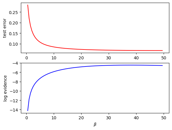
_images/f1c974b1e067eb6a868ffbd202fedd6f539cbf39a4e3777c6011e19a9691e3c3.png

# compare different values of beta
M = 10  # number of basis functions
alpha = 3. 
betas = np.arange(0.5, 50., 0.5)
mse = []  # mean square errors
lev = []  # log evidences
for beta in betas:
    Phi = gbf1(x, [-xr,xr], M)  # Gaussian basis functions
    m, S = blr(Phi, t, alpha, beta)
    lev.append( logev(Phi, t, m, S, alpha, beta))
    # test data
    Phip = gbf1(xp, [-xr,xr], M)  # Gaussian basis functions
    err = fp - Phip@m.T  # validation error
    mse.append( np.dot(err,err)/Np)
    #print(alpha, beta, lev, mse)
plt.subplot(2,1,1)
plt.plot(betas, mse, "r"); plt.ylabel("test error");
plt.subplot(2,1,2)
plt.plot(betas, lev, "b"); plt.ylabel("log evidence");
plt.xlabel(r"$\beta$");

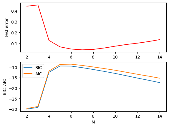
_images/84f0d33aa009f2d36cd69fabac27a10f8e4d1501d8ffe1095cb58898fe8b80e6.png

BIC and AIC#

In addition to the parameters $\alpha$ and $\beta$, we want to select the number $M$ of the basis functions.

The evidence for the model with $M$ parameters trained by $N$ samples are approximated by

\[ \log p(\b{t}|M) \simeq -\frac{\beta}{2} ||\b{t}-X\b{m}||^2 - \frac{1}{2}M\log N \]

This is know as the Bayesian information criterion (BIC). See Bishop Chapter 4.4 for details.

Another popular tool for model selection is Akaike information criterion (AIC), which is given by

\[ AIC = -\frac{\beta}{2} ||\b{t}-X\b{m}||^2 - M. \]

AIC is based on the KL divergence of the data distributions between the true model and learned model.

Let us compare the test error and BIC for different model complexity $M$.

def bic(X, t, m, beta):
    """BIC and AIC
    m: posterior mean
    beta: inv. variance of observation noise
    """
    N, M = X.shape
    em = t - X@m.T  # error with MAP estimate
    # log evidence
    bic = -beta/2*np.dot(em,em) - M/2*np.log(N)
    aic = -beta/2*np.dot(em,em) - M
    return bic, aic

# compare different values of M
Max = 15  # max number of basis functions
alpha = 3.
beta = 20.
mse = np.zeros(Max)  # mean square errors
baic = np.zeros((Max,2))  # log evidences
for M in range(2,Max):
    Phi = gbf1(x, [-xr,xr], M)  # Gaussian basis functions
    m, S = blr(Phi, t, alpha, beta)
    baic[M] = bic(Phi, t, m, beta)
    # test data
    Phip = gbf1(xp, [-xr,xr], M)  # Gaussian basis functions
    err = fp - Phip@m.T  # validation error
    mse[M] = np.dot(err,err)/Np
    # print(M, alpha, beta, lev[M], mse[M])
plt.subplot(2,1,1)
plt.plot(np.arange(2,Max), mse[2:], "r"); plt.ylabel("test error");
plt.subplot(2,1,2)
plt.plot(np.arange(2,Max), baic[2:]); plt.ylabel("BIC, AIC");
plt.legend(("BIC","AIC"))
plt.xlabel("M");

_images/9d5b2ae2d8efaf1bc74101e644d71ec73fae54ba99f861a2693b3080743f01bb.png

Bayesian networks#

As we have seen in the example of Bayesian linear regression, statistical machine learning assumes a generative model of the observed data and infer the posterior probability of variables of your interest, after marginalizing other unobserved variables.

In doing so, representation of the relationships by graphs with random variables as nodes (or vertices) and joint or conditional probabilities as links (or edges or arcs) have turned out to be very useful. They are called graphical models.

Directed graphs representing conditional probabilities by arrows (directed edges) are called Bayesian networks.

For example, Bayesian linear regression can be represented as a Bayesian network as below.

Graphical model for the Bayesian linear regression.

Inference in Bayesian network goes like this: as values of some variables are observed,

clamp the values of the nodes where observation was made.
compute the posterior distributions of the nodes along the graph by repeating Bayesian inference and marginalization

In doing this, the conditional independence of the nodes allows efficient computation.

Inference on a chain#

Here we consider the simplest case of a chain of discrete random variables.

Graphical model of a chain of states.

For each node, the variable takes an integer value $x_n \in \{1,...,K_n\}$ and we consider the joint distribution over the entire nodes:

\[ p(x_1,...,x_N) = p(x_1)p(x_2|x_1) \cdots p(x_{N-1}|x_{N-2})p(x_N|x_{N-1}). \]

When an observation $x_N=k$ is made at the end node, we would consider the posterior distribution

\[ p(x_1,...,x_{N-1}|x_N=k) \propto p(x_1)p(x_2|x_1) \cdots p(x_{N-1}|x_{N-2})p(x_N=k|x_{N-1}). \]

The posterior distribution of each node $x_n$ is given by marginalization

\[ p(x_n|x_N=k) \propto \sum_{x_1}\cdots\sum_{x_{n-1}}\ \sum_{x_{n+1}}\cdots\sum_{x_N}p(x_1,...,x_{N-1}|x_N=k) \]

\[ = \left\{\sum_{x_{n-1}}p(x_n|x_{n-1}) \cdots \sum_{x_1}p(x_2|x_1)p(x_1)\right\} \]

\[ \times \left\{\sum_{x_{n+1}}p(x_{n+1}|x_n) \cdots \sum_{x_{N-1}}p(x_{N-1}|x_{N-2}) \sum_{x_N}p(x_N=k|x_{N-1})\right\} \]

This can be computed efficiently by passing two messages:

Forward message $\alpha_n$ of prior:

\[ \alpha_1 = p(x_1)\]

\[ \alpha_n = \sum_{x_{n-1}} p(x_n|x_{n-1}) \alpha_{n-1} \]

Backward message $\beta_n$ of likelihood:

\[ \beta_N = (0,...,1,...0) \]

with $1$ at $k$-th component and

\[ \beta_n = \sum_{x_{n+1}} p(x_{n+1}|x_n) \beta_{n+1} \]

The posterior distribution for each node is then given by their product

\[ p(x_n|x_N=k) \propto \alpha_n \beta_n. \]

This is called forward-backward algorithm.

This can be generalized to tree-like networks and the algorithm using forward and backward message passing is known as belief propagation.

Markov chain#

Here is an example of inference in a Markov chain.

class Markov:
    """Class for a Markov chain"""
    
    def __init__(self, ptr):
        """Create a new environment"""
        self.ptr = ptr  # transition matrix p(x'|x)
        self.Ns = len(ptr)  # number of states
        
    def sample(self, x0=0, step=1):
        """generate a sample sequence from x0"""
        seq = np.zeros(step+1, dtype=int) # sequence buffer
        seq[0] = x0
        for t in range(step):
            pt1 = self.ptr[:, seq[t]] # prob. of new states
            seq[t+1] = np.random.choice(self.Ns, p=pt1) # sample 
        return seq
    
    def forward(self, p0, step=1):
        """forward message from initial distribution p0"""
        alpha = np.zeros((step+1, self.Ns)) # priors
        alpha[0] = p0  # initial distribution
        for t in range(step):
            alpha[t+1] = self.ptr @ alpha[t] 
        return alpha

    def backward(self, obs, step=1):
        """backward message from terminal observaion"""
        beta = np.zeros((step+1, self.Ns)) # likelihoods
        beta[-1] = obs  # observation
        for t in range(step, 0, -1): # toward 0
            beta[t-1] = beta[t] @ self.ptr
        return beta
    
    def posterior(self, p0, obs, step):
        """forward-backward algorithm"""
        alpha = self.forward(p0, step)
        beta = self.backward(obs, step)
        post = alpha*beta
        for t in range(step+1):
            post[t] = post[t]/sum(post[t])  # normalize        
        return post

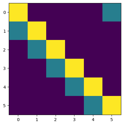
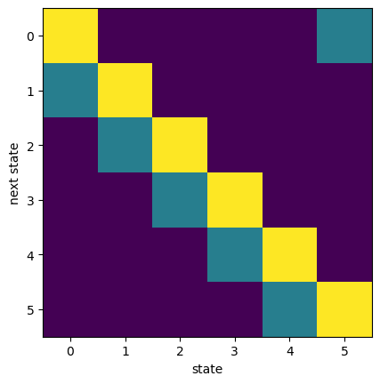
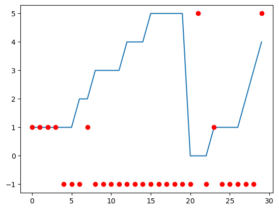
Here is an example of directed random walk on a ring.

# stochastic cycling on a ring
ns = 6   # ring size
ps = 0.3  # shift probability
Ptr = np.zeros((ns, ns))  # transition matrix
for i in range(ns):
    Ptr[i,i] = 1 - ps
    Ptr[(i+1)%ns, i] = ps
plt.imshow(Ptr)
# create a Markov chain
ring = Markov(Ptr)

_images/111a66b931483a9120cb7cf5f88d52b0b9eb535625963aeff88ba2ee52e0fa91.png

# a sample trajectory
T = 15
ring.sample(1, T)

array([1, 1, 1, 1, 2, 3, 3, 3, 3, 3, 3, 4, 4, 4, 4, 5])

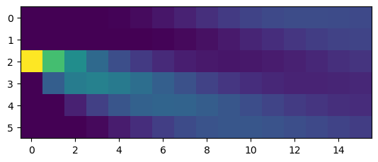
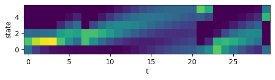
# forward message passing
alpha = ring.forward([0,0,1,0,0,0], T)
plt.imshow(alpha.T);

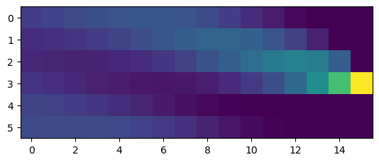
_images/8e088fe7cf1dd80705a6186bdaf9fd64e5a814b6e91a04f541a13fada799b933.png

# backward message passing
beta = ring.backward([0,0,0,1,0,0], T)
plt.imshow(beta.T);

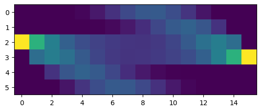
_images/ac0488e366875ac339def9ec78a1a45545bf95ffcbd6d03ff6ddba7665afe8ec.png

# posterior by their products
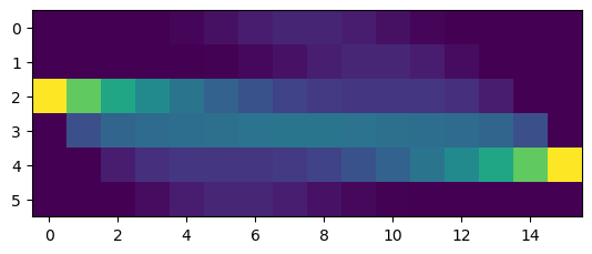
post = ring.posterior([0,0,1,0,0,0], [0,0,0,1,0,0], T)
plt.imshow(post.T);

_images/7935061d131cce2876c40ef17ebb6e2e6ffa26b4edb358b34de183e668dfcb33.png

# a little shifted observation
post = ring.posterior([0,0,1,0,0,0], [0,0,0,0,1,0], T)
plt.imshow(post.T);

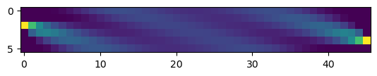
_images/45a7d79066c7237ce7484a277640a9f360fbea0f59acee8b89fc231ee31c5445.png

# longer sequence
post = ring.posterior([0,0,1,0,0,0], [0,0,0,0,1,0], 3*T)
plt.imshow(post.T);

_images/4d10a1f21f9753b8424dee45ae9d1fc7d9a015717adc492abd6a0c0760a96450.png

Dynamic Bayesian Inference#

Iterative Bayesian inference can be generalized to the case when the hidden variable $x$ changes dynamically.

We denote the sequence of observation as

\[ y_{1:t}=(y_1,..,y_t) \]

and the history of underlying state variable as

\[ x_{1:t}=(x_1,..,x_t). \]

We assume two conditional probability distributions:

Dynamics model: $p(x’|x)$
Observation model: $p(y|x)$

Using the posterior $p(x_t|y_{1:t})$ computed from the data up to time $t$, we use the dymamics model to compute the predictive prior:

\[ p(x_{t+1}|y_{1:t}) = \int p(x_{t+1}|x_t) p(x_t|y_{1:t}) dx_t \]

by integrating or summing over the possible range of $x$.

We can combine this prior with the new coming data $y_{t+1}$ to update the posterior as:

\[ p(x_{t+1}|y_{1:t+1}) = \frac{p(y_{t+1}|x_{t+1}) p(x_{t+1}|y_{1:t})}{ p(y_{1:t+1})}. \]

This is called dynamic Bayesian inference and allows real-time tracking of hidden variables from noisy observations.

When $x$ is discrete, the process is called hidden Markov model (HMM), which has been used extensively speech processing.

Another example is Kalman filter, in which $x$ and $y$ are continuous and the dynamics and observation models are linear mapping with Gaussian noise.

Hidden Markov model#

Here is a simple implementation of HMM based on the Markov chain above.

class HMM(Markov):
    """Hidden Markov model"""

    def __init__(self, ptr, pobs):
        """Create HMM with transition and observation models"""
        super().__init__(ptr)
        self.pobs = pobs  # observation model
        self.No = len(pobs)  # number of observations
        self.pst = np.ones(self.Ns)/self.Ns  # state distribution
        self.pred = np.zeros(self.Ns)  # predictive distribution

    def sample(self, x0=0, step=10):
        """generate a sample sequence from x0"""
        xt = np.zeros(step, dtype=int) # state sequence
        yt = np.zeros(step, dtype=int) # observation sequence
        xt[0] = x0
        po = self.pobs[:, x0] # prob. of observation
        yt[0] = np.random.choice(self.No, p=po) # observe
        for t in range(1, step):
            ps = self.ptr[:, xt[t-1]]  # prob. of new states
            xt[t] = np.random.choice(self.Ns, p=ps) # transit 
            po = self.pobs[:, xt[t]]   # prob. of observation
            yt[t] = np.random.choice(self.No, p=po) # observe 
        return xt, yt

    def predict(self):
        """predictive prior by transition model"""
        self.pred = self.ptr @ self.pst
    
    def update(self, obs):
        """update posterior by observation"""
        prl = self.pobs[obs]*self.pred # likelihood*prior
        self.pst = prl/sum(prl)  #normalize

    def reset(self):
        """reset state probability"""
        self.pst = np.ones(self.Ns)/self.Ns  # uniform

    def step(self, obs):
        """one step of dynamic bayesian inference"""
        self.predict()
        self.update(obs)
        return self.pst  # new prior

Here is an example of directed random walk on a ring, like a mouse walking on a circular track.

# random walk on a ring
ns = 6   # ring size
ps = 0.3  # shift probability
Ptr = np.zeros((ns, ns))  # transition matrix
for i in range(ns):
    Ptr[i,i] = 1 - ps
    Ptr[(i+1)%ns, i] = ps
plt.imshow(Ptr)
plt.xlabel("state"); plt.ylabel("next state");

_images/0f12002896f1979b7222832735a44c6012a71a31536c6bf7a564a599b00e6ec7.png

Suppose we have three coarse position sensors, which send signal only intermittently, and we want to estimate where the mouse is.

# Blurred intermittent observation model
no = 4
po = 0.3
Pobs = np.zeros((no, ns))  # p(obs|state)
Pobs[0,:] = 1 - po  # no information
Pobs[1,1] = Pobs[2,3] = Pobs[3,5] = po
Pobs[1,0] = Pobs[3,0] = Pobs[1:3,2] = Pobs[2:4,4] = po/2
plt.imshow(Pobs)
plt.xlabel("state"); plt.ylabel("observation");

_images/ba7cfa8bc71cd102c039d7d7e9a50eb69b8a00cef9028a00ae41f02e7249ddc6.png

# crate a HMM
ring = HMM(Ptr, Pobs)

# sample a state trajectory and observations
T = 30
xt, yt, = ring.sample(1, T)
plt.plot(xt)
plt.plot(2*yt-1, 'ro');

_images/714feeb7954002608a74d7836db3d588313c4dd7f7af0f432b5116ce02d16ac1.png

From such noisy intermittent observations, how can we estimate the state?

# Dynamic Bayesian inference in HMM
post = np.zeros((T, ns))  # posterior trajectory
ring.reset()
for t in range(T):
    post[t] = ring.step(yt[t])
plt.imshow(post.T, origin='lower')
plt.xlabel('t'); plt.ylabel('state');

_images/fd9325b61ba36ab6c1bc9f0bf4c667b808fcb5b8e41f0e0a36a77dbfd7db002f.png

Even when there is no useful sensory input, you can predict the state distribution by the dynamic model. When a sensory input becomes available, prediction is corrected and sharpened.

After sensory input, you can also reflect back and consider which previous states were more likely using forward-backward algorithms.

Approximate Bayesian inference#

For discrete distributions and continuous distributions following Gaussians and some others, computation of posterior distribution is not too difficult.

For example, if the likelihood function and the prior distribution follow certain distributions like Gaussian, we can just keep track of the parameters of the distribution and the normalizing factor is given analytically. For example, if both the likelihood and the prior and Gaussian, we can match the second and first-order coefficients of the exponent as $-\frac{1}{2\sigma^2}$ and $\frac{\mu}{\sigma^2}$ and then the normalizing factor is analytically given as $\sqrt{2\pi\sigma^2}$.

But when we deal with an arbitrary high-dimension continous distributions, computation of posterior distribution. Especially the computation of the normalizaing factor (marginal likelihood) can be quite hard for integration over multiple dimensions.

For such cases, there are approximate Bayesian inference methods, such as variational inference and sampling methods.

Variational inference#

In variational inference, we approximate the posterior distribution by a certain functional form $q(x)$, and update it to minimize the discrepancy from the posterior distribuion, usually measured by the KL divergence

\[ KL[q(x);p(x|y)] = \int q(x) \log\frac{q(x)}{p(x|y)} dx \]

A typical assumption is that the posterior distribution can be factorized, i.e. represented by a product of distributions of different groups

\[ q(x) = \prod_i q_i(x_i). \]

This leads to an repeated alternating optimization similar to the EM algorithm, but by taking into account the distribution of each group of variables.

See Chapter 10 of Bishop (2006) for details.

Sampling methods:#

In the sampling methods, we approximate a distribution $p(x)$ by a collection of points $\{x_1,...,x_n\}$.

We are often interested in evaluating the expectation of a certain function over the posterior distribution

\[ E_{p(x)}[f(x)] = \int f(x)p(x) dx \]

This can be approximated by the sum of the values at the sample points

\[ E_{p(x)}[f(x)] = \frac{1}{n} \sum_{i=1}^n f(x_i) \]

if the distribution of samples ${x_i}$ well approximates $p(x)$.

Markov chain Monte Carlo (MCMC)#

Markov chain Monte Carlo (MCMC) takes a new sample near the previous sample and accept or reject it based on unnormalized correlates of the target probability, such as the product of the likelihood and the prior, so that the sequence of samples follows the target distribution, such as the posterior distribution in Bayesian inference.

A simple example of MCMC is Metropolis sampling, which requires only unnormalized propability $\tilde{p}(x)\propto p(x)$ of samples for relative comparison.

A new candidate $x^*$ is generated by a symmetric proposal distribution $q(x^*|x_k)=q(x_k|x^*)$, such as a gaussian distribution, and acctepted with the probability

\[ p_\mbox{acc} = \min(1, \frac{\tilde{p}(x^*)}{\tilde{p}(x_k)}) \]

def metropolis(p, x0, sig=0.1, m=1000):
    """metropolis: Metropolis sampling
    p:unnormalized probability, x0:initial point,
    sig:sd of proposal distribution, m:number of sampling"""
    n = len(x0)  # dimension
    p0 = p(x0)
    x = []
    for i in range(m):
        x1 = x0 + sig*np.random.randn(n)
        p1 = p(x1)
        pacc = min(1, p1/p0)
        if np.random.rand()<pacc:
            x.append(x1)
            x0 = x1
            p0 = p1
    return np.array(x)

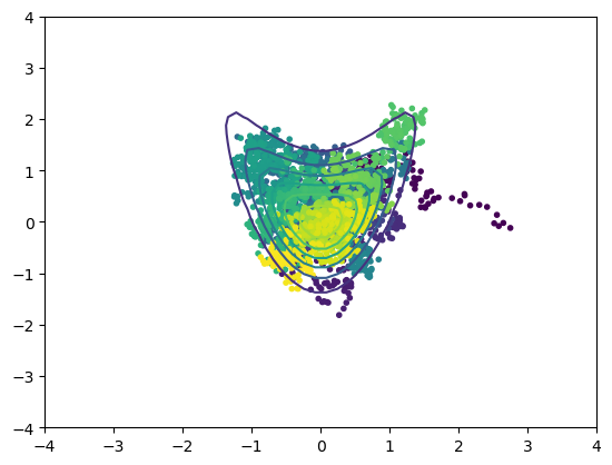
def croissant(x):
    """croissant-like unnormalized distribution in 2D"""
    return np.exp(-x[0]**2 - (x[1]-x[0]**2)**2)

r = 4  # plot rage
x = np.linspace(-r, r)
X, Y = np.meshgrid(x, x)
P = croissant(np.array([X,Y]))
plt.contour(X, Y, P)  # target
x = metropolis(croissant, [3,0], sig=0.1, m=3000)
s = len(x); print(s)  # accepted samples
plt.scatter(x[:,0], x[:,1], c=np.arange(s), marker='.');

_images/804e5fa7280fff56a0de123ab4dfc50b80862272440aba5e4d831dcae0cbdbb6.png

Bayesian sensorimotor processing#

Our life is full of uncertainty. In sensory perception, we need to cope with noise, delay and occulusion and also overcome fundamental ill-posedness, such as to identify the 3D location of your target from 2D retinal images or sounds to two ears.

To find a practical solution to such ill-posed problems, we need to make use of some prior assumptions, such as the light usually comes from the top or objects don’t jump abruptly.

Bayesian inference provides a principled way for combining any prior knowledge with sensory evidence. Indeed there are several lines of psychological evidence suggesting that humans and animals integrate knowledge from prior experience or multi-modal sensory information as predicted by Bayesian inference (Knill & Pouget 2004, Doya et al. 2007).

Ernst & Banks (2002) tested in a grasping task in a virtual reality setting how human subjects’ object size perception depends on the noise level in the visula feedback. They showed that as the viaual noise increases, subjects’ responses are closer to the size estimated by the haptic input, consistently with the ratio of the variances or visual and haptic perception as predicted by the Bayesian theory of multisensory integration.
Kording & Wolpert (2004) tested in an arm reaching task with modified visual feedback how the prior expectation based on repeated trials is combined with visual feedback of different clarities upon each trial. They showed that the subjects’ performance was based more on the visual feedback for higher clarity, as expected from Bayesian integration of the prior and likehihood by their variances.

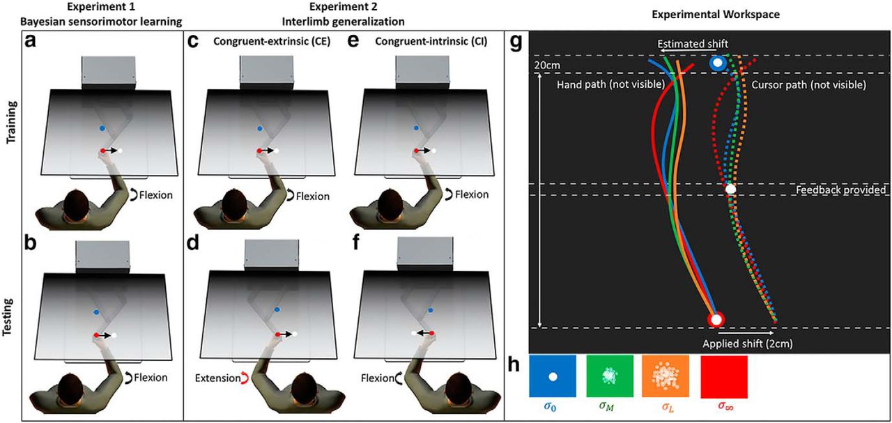
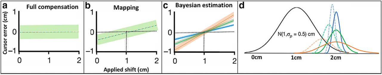
This is a study by Hewitson et al. (2018) following the experiment by Wolpert & Koerding (2004). As the subject tries to move the cursor to the target, a random shift is introduced to the hand-to-curs mapping. The subjects acquire a prior distribution of the cursor shift from experience, and combine that with sensory feedback with different clarities in the middle of reaching. They confirmed that the subjects’ performance followed the predicted by Bayesian inference and further showed that the performace generalize across the arm used (from Hewitson et al. 2018).

Bayesian computation in the brain#

How such Bayesian computation realized in the brain? How does the brain represent and manipulate probability distributions?

One possibility is that the receptive field of a neuron represents a basis function in the sensory space and the activities of a population of neurons represent a probability distribution. This idea is called probabilistic population code (Zemel et al. 2004, Ma et al. 2006).

The cerebral cortex has a hierarchical organization and bi-directional connections between lower and higher areas originating from specific layers. There have been serveral hypotheses about how such hierarchical recurrent network can realize Bayesian inference, such as by belif propagation (Lochmann & Deneve 2011; George D, Hawkins J 2009).

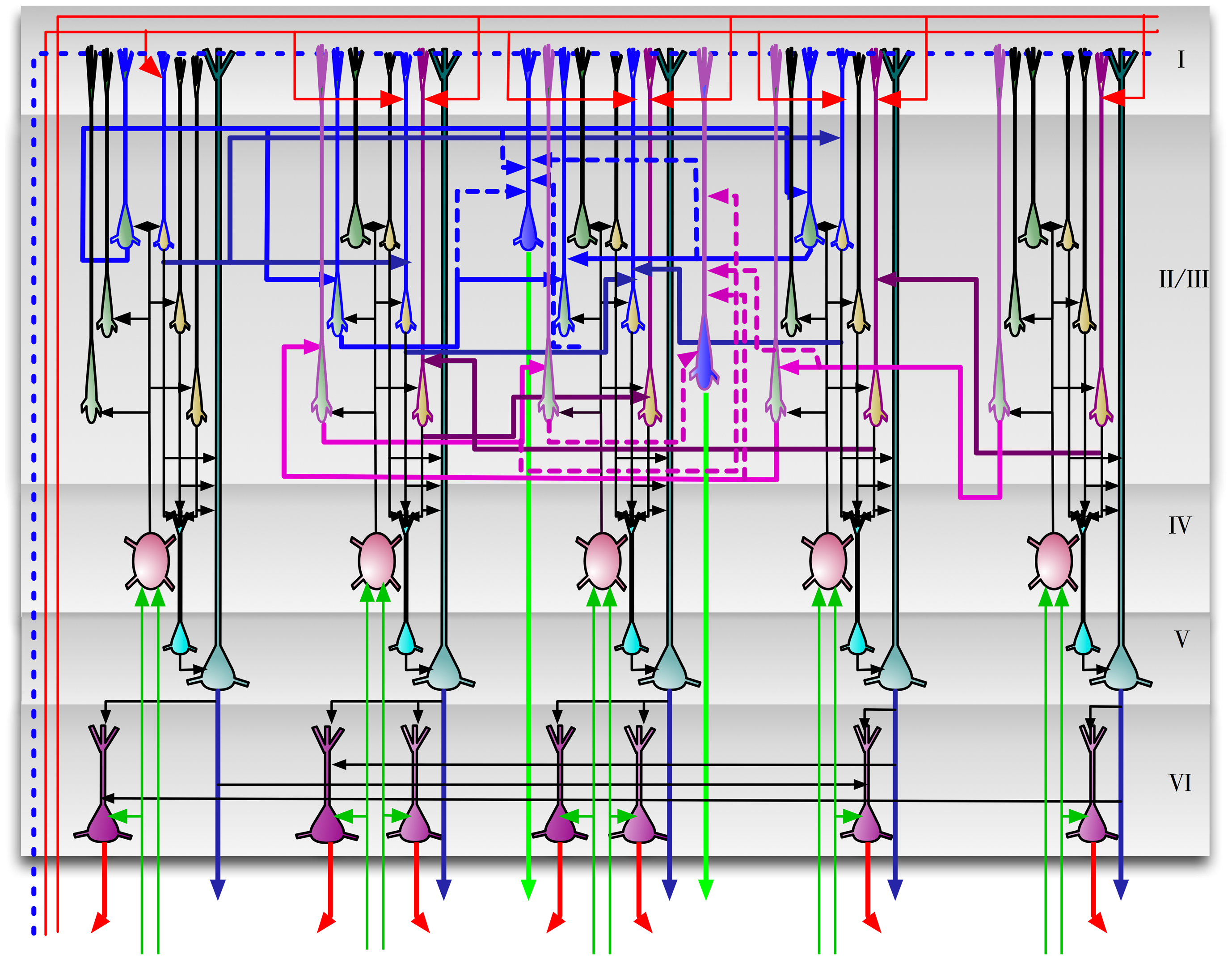
A hypothetical diagram of how bottom-up (green) and top-down (red) messages for Bayesian inference are processed by neurons in different cortical layers. From George and Hawkins (2009).

Karl Frisont considered variational approximation as a plausible mechanism of Bayesian inference in the brain and proposed the minimization of variational free energy as the basic operational principle of the brain (Friston 2005, 2010). His group proposed how such operations can be implemented in the canonical cortical circuits (Bastos et al. 2012).

Bastos and colleagues proposed a hypothesis about how Bayesian inference by variational approximation, know as predictive coding can be implemented in the canonical cortical circuits (from Bastos et al., 2012)

Experimental investigation of Bayesian inference in the brin#

To test the hypotheses that cortical circuits perform dynamics Bayesian inference, Funamize et al. (2016) trained mice to navigate in an auditory virtual environment with head fixed and performed calcium imaging of neurons in the parietal cortes by a two-photon microscope. Bayesian decoding of neural population activity by the method of Ma et al. (2006) showed that the inferred goal distance reduced even while auditory feedback was turned off, presumably by using action-dependent state transition model, and the variace of the goal distance was reduced as the auditory feedback was turned on again, similar to the feature of dynamic Bayesian inference.

Left: goal distance tuning of recorded neurons. Right: from the instantaneous observation of the population neural activity, by combination of the likelihoods and a flat prior, the posterior distribution of the goal distance was computed by probabilistic population coding model (Ma et al, 2006). The posterior distribution shifted even when the sound feedback was turoen off (between red bars), and the distribution became sharper when the sound feedback was turned on (red bar). From Funamizu et al. (2016)

References#

Bishop CM (2006) Pattern Recognition and Machine Learning. Springer. https://www.microsoft.com/en-us/research/people/cmbishop/prml-book/
- Chapter 3: Bayesian linear regression
- Chapter 8: Graphical models
- Chapter 10: Approximate Bayesian inference
- Chapter 11: Sampling methods

Bayesian sensorimotor integration#

Knill DC, Pouget A (2004) The Bayesian brain: the role of uncertainty in neural coding and computation. Trends in neurosciences 27:712-719. https://doi.org/10.1016/j.tins.2004.10.007
Doya K, Ishii S, Pouget A, Rao R (2007) Bayesian Brain: Probabilistic Approach to Neural Coding and Learning. MIT Press.
Ernst MO, Banks MS (2002). Humans integrate visual and haptic information in a statistically optimal fashion. Nature, 415, 429-433. https://doi.org/10.1038/415429a
Körding KP, Wolpert DM (2004) Bayesian integration in sensorimotor learning. Nature 427:244-247. https://doi.org/10.1038/nature02169
Hewitson CL, Sowman PF, Kaplan DM (2018). Interlimb Generalization of Learned Bayesian Visuomotor Prior Occurs in Extrinsic Coordinates. eneuro, 10.1523/eneuro.0183-18.2018. https://doi.org/10.1523/eneuro.0183-18.2018

Probabilistic population codes#

Zemel RS, Dayan P, Pouget A (1998) Probabilistic interpretation of population codes. Neural computation 10:403-430. https://doi.org/10.1162/089976698300017818
Ma WJ, Beck JM, Latham PE, Pouget A (2006) Bayesian inference with probabilistic population codes. Nature neuroscience 9:1432-1438. https://doi.org/10.1038/nn1790

Baysian inference in the cortical circuit#

George D, Hawkins J (2009). Towards a mathematical theory of cortical micro-circuits. PLoS Comput Biol, 5, e1000532. https://doi.org/10.1371/journal.pcbi.1000532
Lochmann T, Deneve S (2011) Neural processing as causal inference. Current opinion in neurobiology 21:774-781. https://doi.org/10.1016/j.conb.2011.05.018
Friston K (2005). A theory of cortical responses. Philos Trans R Soc Lond B Biol Sci, 360, 815-36. http://doi.org/10.1098/rstb.2005.1622
Friston K (2010). The free-energy principle: a unified brain theory? Nat Rev Neurosci, 11, 127-38. http://doi.org/10.1038/nrn2787
Bastos AM, Usrey WM, Adams RA, Mangun GR, Fries P, Friston KJ (2012). Canonical microcircuits for predictive coding. Neuron, 76, 695-711. https://doi.org/10.1016/j.neuron.2012.10.038
Bogacz R (2017) A tutorial on the free-energy framework for modelling perception and learning. Journal of Mathematical Psychology. 76, 198–211. https://doi.org/10.1016/j.jmp.2015.11.003
Funamizu A, Kuhn B, Doya K (2016) Neural substrate of dynamic Bayesian inference in the cerebral cortex. Nature Neuroscience 19:1682-1689. https://doi.org/10.1038/nn.4390

\(p(Y \vert X)\)	no mouse \(X=0\)	mouse hiding \(X=1\)
no sound \(Y=0\)	0.9	0.5
sound \(Y=1\)	0.1	0.5