Chapter 5. Unsupervised Learning#
Contents#
Clustering (Bishop, Chater 9):
\(k\)-means clustering
mixtures of Gaussians
self-organizing maps (SOM)
Subspace mapping (Biship, Chapter 12):
principal component analysis (PCA)
singular value decomposition (SVD)
independent component analysis (ICA)
Neural Mechanisms
Receptive field formation
As we grow, we learn that there are different things and creatures in the world, such as plants and animals, and in more detail, dogs, cats and humans. What is remarkable is that most of such learning is done spontaneously without explicit teaching about what is a dog, or labels specifying which is a dog or which is a cat.
Learning categories without explicit labels is an example of unspervised learning.
The key in unsupervised learning is to find a certain structure in the distribution of the observed data \(\{\b{x}_1,...,\b{x}_N\}\), and come up with a probabilistic model \(p(\b{x})\) that produced the data.
Typical cases are:
Dividing into clusters:
\(k\)-means clustering
mixtures of Gaussians
hierarchical clustering
Decomposing into components:
principal component analysis (PCA)
singular value decomposition (SVD)
independent component analysis (ICA)
import numpy as np
import matplotlib.pyplot as plt
%matplotlib inline
scikit-learn#
scikit-learn is a popular Pyhon libraries of supervised and unsupervised learning algorithms and sample datasets.
You can explore the algorithms in the tutorial: tutorials
Here we take a classic dataset iris from scikit-learn.
from sklearn import datasets
# the iris dataset
iris = datasets.load_iris()
#print(iris.DESCR)
X = iris.data  # flower features
C = iris.target  # flower class
N, D = X.shape
print(N, D)
150 4
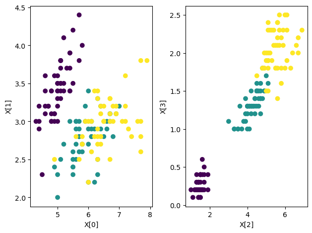
Here is a visualization of the 4D data in 2D each.
plt.subplot(1, 2, 1)
plt.scatter(X[:,0], X[:,1], c=C);  # sepal length, width
plt.xlabel('X[0]'); plt.ylabel('X[1]');
plt.subplot(1, 2, 2)
plt.scatter(X[:,2], X[:,3], c=C);  # petal length, width
plt.xlabel('X[2]'); plt.ylabel('X[3]');
plt.tight_layout();
K-means Clustering#
The most basic method of clustering is \(K\)-means clustering, which divides a data set \(\{\b{x}_1,…,\b{x}_N\}\) into \(K\) clusters.
We define prototypes \(\b{\mu}_k\) for \(k=1,...,K\) clusters and specify belonging of data points by binary indicator variables \(r_{nk}\in\{0,1\}\).
A good clustering is achieved by minimizing the distortion measure
which is a sum of distances of the data point from its prototype.
We do that by repeating the following steps:
For the current prototypes \(\b{\mu}_k\), re-assign each data point \(\b{x}_n\) by finding the nearest \(\b{\mu}_k\) and setting \(r_{nk} = 1\) and \(r_{n j\ne k} = 0\).
For the current assignment by \(r_{nk}\), update the prototypes by
Here is a sample implementation of K-means.
class KMeans:
    """K-Means clustering"""
    def __init__(self, data, K=2):
        """data: NxD data matrix
        K: number of clusters"""
        self.X = data  # store dataset
        self.N, self.D = data.shape  # data dimensions
        self.K = K  # number of clusters
        self.C = np.zeros(self.N, dtype=int)   # cluster indices for data points
        self.R = np.zeros((self.N,self.K), dtype=int)   # indicator matrix
        self.Mu = data[np.random.randint(0, self.N, self.K),:]   # pick K points randomly

    def update(self):
        # Re-assign to clusters
        self.R[:] = 0  # clear the indicator variables
        for n in range(self.N):
            # check the distances
            dist = [ np.sum((self.X[n]-self.Mu[k])**2) for k in range(self.K)]
            # find the nearest mean
            self.C[n] = np.argmin(dist)  # new cluster assignment
            self.R[n, self.C[n]] = 1  # new indicator variable
        # Update the means
        for k in range(self.K):
            self.Mu[k] = self.R[:,k]@self.X/np.sum(self.R[:,k])

    def run(self, imax=20):
        """repeat until convergence"""
        for i in range(imax):
            R0 = self.R.copy() # previous indicators
            self.update()
            if np.array_equal(self.R, R0):
                print('converged with iteration', i)
                break
        return self.C, self.R, self.Mu
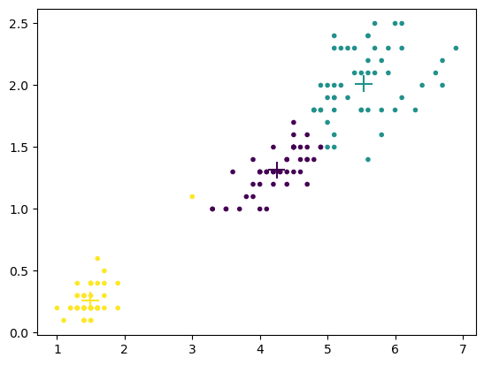
Try applying it to the last 2D of the iris dataset for easy visualization.
# initialize the algorithm
km = KMeans(X[:,2:], K=3)
print( km.N, km.D, km.K)
150 2 3
# See step by step
km.update()
#print(km.C)
plt.scatter(X[:,2], X[:,3], c=km.C, marker='.')  # data colored by cluster
plt.scatter(km.Mu[:,0], km.Mu[:,1], c=range(km.K), marker='+', s=200);  # means
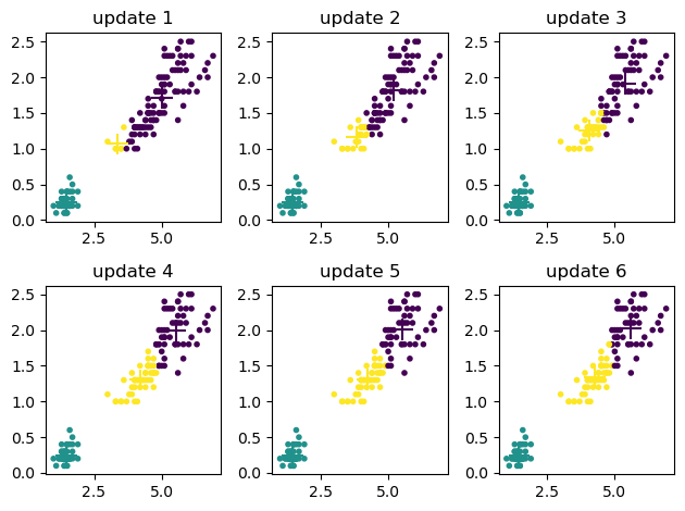
km = KMeans(X[:,2:], K=3)
up = 6  # updates
for u in range(up):
    km.update()
    plt.subplot(2, int(np.ceil(up/2)), u+1)
    plt.title(f"update {u+1}")
    plt.scatter(X[:,2], X[:,3], c=km.C, marker='.')  # data colored by cluster
    plt.scatter(km.Mu[:,0], km.Mu[:,1], c=range(km.K), marker='+', s=200)  # means
plt.tight_layout()
print(km.C)
[1 1 1 1 1 1 1 1 1 1 1 1 1 1 1 1 1 1 1 1 1 1 1 1 1 1 1 1 1 1 1 1 1 1 1 1 1
 1 1 1 1 1 1 1 1 1 1 1 1 1 2 2 2 2 2 2 2 2 2 2 2 2 2 2 2 2 2 2 2 2 2 2 2 2
 2 2 2 0 2 2 2 2 2 0 2 2 2 2 2 2 2 2 2 2 2 2 2 2 2 2 0 0 0 0 0 0 2 0 0 0 0
 0 0 0 0 0 0 0 0 0 0 0 0 0 0 0 2 0 0 0 0 0 0 0 0 0 0 0 2 0 0 0 0 0 0 0 0 0
 0 0]
Please try K smaller or larger than 3, or original 4D space.
Mixtures of Gaussians#
It is often the case that clusters have some overlaps and assignment is probabilistic. Mixtures of Gaussians is a probabilistic extention of \(K\)-means clustering.
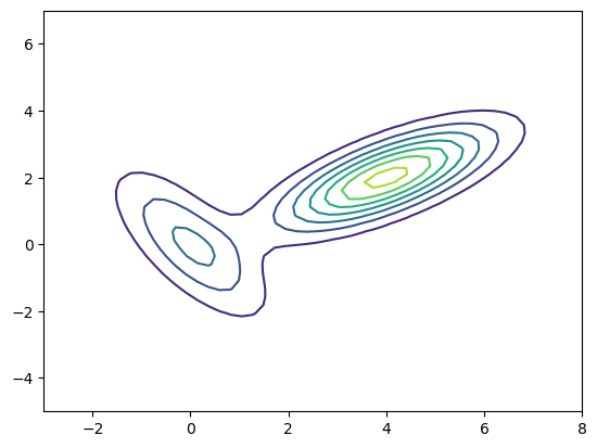
Gaussian mixture distribution has a form
where \(\b{\mu}_k\) and \(\Sigma_k\) are the mean vector and the covariance matrix of \(k\)-th Gaussian distribution and \(\pi_k\) is the mixture probability.
The probability density function (PDF) of a d-dimension Gaussian distribution is given by:
Here we use the multivariate_normal function in scipy to visualize the PDF of a Mixture of Gaussians.
from scipy.stats import multivariate_normal
# Probability density of a Mixture of Gaussians
def mixgauss_pdf(x, pi, mu, sigma):
    K, D = np.array(mu).shape  # classes and data dimension
    p = np.zeros(x.shape[:-1])
    for k in range(K):
        p += pi[k]*multivariate_normal.pdf(x, mu[k], sigma[k])
    return p
pi = [0.3, 0.7]    # mixture probability
mu = [[0,0], [4,2]]     # means
sigma = [[[1,-1],[-1,2]], [[2,1],[1,1]]]   # variances
x0 = np.linspace(-3, 8)
x1 = np.linspace(-5, 7)
X0, X1 = np.meshgrid(x0, x1)
P = mixgauss_pdf(np.stack((X0,X1), axis=2), pi, mu, sigma)
plt.contour(X0, X1, P);
Let us generate data from this Mixture Gaussian.
# sample from a Mixture Gaussian distribution
def mixgauss_sample(pi, mu, sigma):
    K = len(pi)
    k = np.random.choice(K, p=pi)
    x = np.random.multivariate_normal(mu[k], sigma[k])
    return x, k
N = 500
X = np.zeros((N,2))
C = np.zeros(N, dtype=int)
for n in range(N):
    X[n,:], C[n] = mixgauss_sample(pi, mu, sigma)
plt.contour(X0, X1, P);
plt.scatter(X[:,0], X[:,1], c=C, marker='.');

Expectation-Maximization (EM) Algorithm#
For finding the parameters \(\pi_k\), \(\mu_k\) and \(\Sigma_k\) \((k=1,...,K)\) for a give dataset, a standard way is to repeat the following steps, called the expectation-maximization (EM) algorithm:
E (expectation) step#
We consider a binary stochastic variable
where \(z_k\in\{0,1\}\) and \(\sum_{k=1}^K z_k=1\), indicating which Gaussian a data point belongs to.
For the current parameters \((\pi_k,\mu_k\),\(\Sigma_k)\), evaluate the posterior probability of \(\b{z}\) from the prior probability \(\pi\) and the likelihood for the data \(\b{x}\), called responsibility:
M (maximization) step#
For the current responsibility, update the parameters as the maximum likelihood estimate for the data weighted by the responsibility:
class MixGauss:
    """MixGauss: Mixture of Gaussians"""
    def __init__(self, data, K=2):
        """X: NxD data matrix
        K: number of Gaussians"""
        self.X = data
        self.N, self.D = data.shape
        self.K = K
        self.Pi = np.ones(self.K)/self.K   # cluster probability
        self.R = np.zeros((self.N,self.K))   # responsibility matrix
        self.Mu = data[np.random.randint(0, self.N, self.K),:]   # pick K points randomly
        self.Sig = np.repeat(np.cov(data.T).reshape(1,self.D,self.D), self.K, axis=0)   # covariance for entire data

    def update(self):
        pr = np.zeros(self.K)   # data probability for each cluster
        """EM update"""
        # Expectation step
        for n in range(self.N):
            for k in range(self.K):
                pr[k] = multivariate_normal.pdf(self.X[n], self.Mu[k], self.Sig[k])
            # responsibility
            self.R[n,:] = pr/np.sum(pr)    # responsibility p(z)
        # Maximization step
        num = np.sum(self.R, axis=0);    # effective numbers for each class
        self.Pi = num/self.N    # class prior
        for k in range(self.K):
            self.Mu[k,:] = np.sum(self.R[:,k]*self.X.T, axis=1)/num[k]
            dX = self.X - self.Mu[k,:]
            self.Sig[k] = self.R[:,k]/num[k]*dX.T@dX  # cluster covariance

    def fit(self, imax=100, conv=1e-6):
        """repeat until convergence"""
        for i in range(imax):
            R0 = self.R.copy()
            self.update()
            #print(self.R, R0)
            if np.sum(abs(self.R-R0))/self.N < conv:
                print('converged with iteration', i)
                break
        return self.R, self.Mu, self.Sig
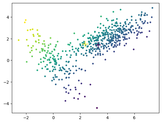
mg = MixGauss(X, 2)
mg.update()
#print("mu =", mg.Mu, "\nsig = ", mg.Sig)
plt.scatter(X[:,0], X[:,1], c=np.dot(mg.R,np.arange(mg.K)), marker='.');
plt.scatter(mg.Mu[:,0], mg.Mu[:,1], c=range(mg.K), marker='+', s=200);  # means
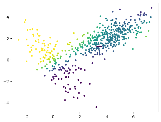
mg.fit()
plt.scatter(X[:,0], X[:,1], c=np.dot(mg.R,np.arange(mg.K)), marker='.');
plt.scatter(mg.Mu[:,0], mg.Mu[:,1], c=range(mg.K), marker='+', s=200);  # means
converged with iteration 83
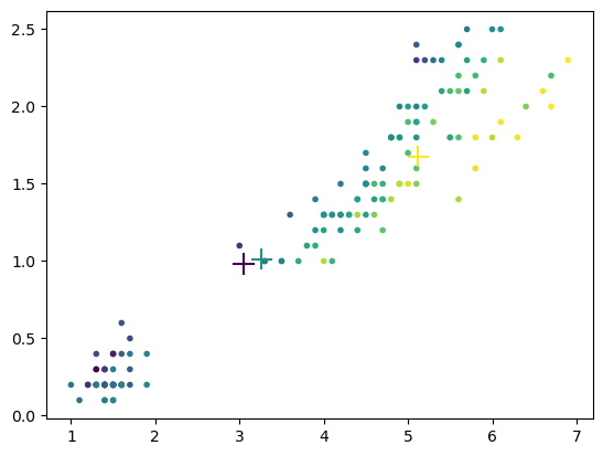
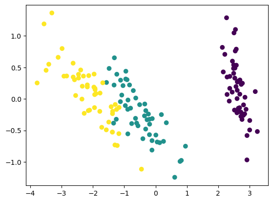
Let us try with the iris dataset.
X = iris.data  # flower features
C = iris.target  # flower class
mg = MixGauss(X, 3)
mg.update()
plt.scatter(X[:,2], X[:,3], c=np.dot(mg.R,np.arange(mg.K)), marker='.');
plt.scatter(mg.Mu[:,2], mg.Mu[:,3], c=range(mg.K), marker='+', s=200);  # means
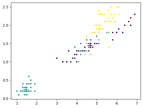
mg.fit()
plt.scatter(X[:,2], X[:,3], c=np.dot(mg.R,np.arange(mg.K)), marker='.');
plt.scatter(mg.Mu[:,2], mg.Mu[:,3], c=range(mg.K), marker='+', s=200);  # means
converged with iteration 79
Dirichlet Process Mixture#
One problem in \(K\)-means and Mixture of Gaussians is that you have to assume the number of clusters \(K\) beforehand.
There is an extension called Dirichlet process mixture that decides the number of clusters based on the data. See Kevin Murphy (2012) Ch. 25.2 for details.
It is available from scikit-learn as mixture.BayesianGaussianMixture
Hierarchical clustering#
Another popular clustering algorithm is hierarchical clustering, which makes a cluster by the closest pair and gradually grow clusters. The results are often shown by a dendrogram*.
These are available in scipy as cluster.hierarchy.
Principal Component Analysis#
Grasping the distribution of a high-dimensional data is not easy for human eyes. We often try to find a low-dimensional projection of the data that characteirizes the distribution.
Principal componet analysis (PCA) finds the directions of the data distribution with the largest variance.
Consider a projection of \(D\)-dimensional vector \(\b{x} = (x_1,...,x_D)^T\) to \(M\)-dimensional vector \(\b{y} = (y_1,...,y_M)^T\) by
where \(V = (\b{v}_1,...,\b{v}_M)^T \in\mathbb{R}^{M\times D}\), \(||\b{v}_m||=1\).
For a data set \(X=(x_1,...,x_N)^T\in\mathbb{R}^{N\times D}\) with zero mean (mean subtracted), we try to find the projection by \(V\) that make the variance of \(\b{y}\) the largest.
Using the covariance matrix of the original data
the covariance matrix of the projected data \(Y=X V^T\) is given as
The variance of projected data is maximized by solving the eigenvalue problem \(C\b{v}=\lambda \b{v}\) and setting the projection matrix \(V=(\b{v}_1,...,\b{v}_M)^T\) made of the eigenvectors with the largest eigenvalues \(\lambda_1,...,\lambda_M\).
# sklearn.datasets offers a wide range of public datasets
from sklearn import datasets
# the iris dataset
iris = datasets.load_iris()
X = iris.data  # flower features
T = iris.target  # flower types
N, D = X.shape
print(N, D)
150 4
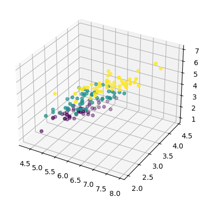
# plot the data in 3D
from mpl_toolkits.mplot3d import Axes3D # for 3D plotting
fig = plt.figure()
ax = fig.add_subplot(111,projection='3d')
ax.scatter(X[:,0], X[:,1], X[:,2], c=T);
# Data covariance
X = X - np.mean(X, axis=0)  # subtract the mean
C = X.T@X/N
# eigenvalue L[i] and normal eigenvector V[:,i]
L, Vt = np.linalg.eigh( C)   # for symmetric matrix
#L, V = linalg.eig( C)
# in matrix form: C*V=V*L, i.e. C=V*L*V' from V'*V=I
print(L)   # eigenvalues
print(Vt)   # columns are eigenvectors
[0.02367619 0.0776881  0.24105294 4.20005343]
[[ 0.31548719  0.58202985  0.65658877 -0.36138659]
 [-0.3197231  -0.59791083  0.73016143  0.08452251]
 [-0.47983899 -0.07623608 -0.17337266 -0.85667061]
 [ 0.75365743 -0.54583143 -0.07548102 -0.3582892 ]]
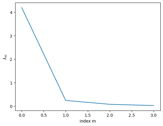
ind = np.argsort(-L)  # largest first
L = L[ind]  # reorder
V = Vt.T[ind]
print(V)
plt.plot(L)
plt.xlabel("index m")
plt.ylabel(r"$\lambda_m$");
[[-0.36138659  0.08452251 -0.85667061 -0.3582892 ]
 [ 0.65658877  0.73016143 -0.17337266 -0.07548102]
 [ 0.58202985 -0.59791083 -0.07623608 -0.54583143]
 [ 0.31548719 -0.3197231  -0.47983899  0.75365743]]
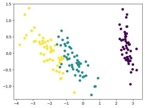
# Projection of data to the PC space
Z = X@V.T
# First two PC
plt.scatter(Z[:,0], Z[:,1], c=T);
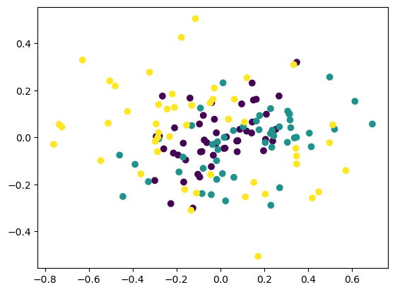
# Last two PC
plt.scatter(Z[:,2], Z[:,3], c=T);
Singular value decomposition (SVD)#
Singular value decomposition (SVD) tries to represent a \(N\times D\) matrix (\(N>D\)) by a weighted sum of products of column vectors \(\b{u}_i \in\mathbb{R}^N\) and row vectors \(\b{v}_i^T \in\mathbb{R}^D\). For example, data may be a mixture of specific patterns \(\b{v}_i\) following certain time courses \(\b{u}_i\).
The decomposition is represented as
where
This decomposition is achieved by selecting \(\b{v}_i\) as the eigenvectors of \(X^T X\) and \(s_i= \sqrt{\lambda_i}\) by their corresponding eigenvalues (\(\lambda_1 \ge ... \ge\lambda_D\)).
Because \(V\) is the same as that for PCA, the SVD algorithm can also be used for PCA.
# X = U*S*V' where S is a diagonal matrix
# i.e. C = X'*X/N = V*S^2/N*V'
U, S, Vs = np.linalg.svd(X)
# See if they match those derived from covariance matrix
print(S**2/N)
print(L)
print(Vs)
print(V)
[4.20005343 0.24105294 0.0776881  0.02367619]
[4.20005343 0.24105294 0.0776881  0.02367619]
[[ 0.36138659 -0.08452251  0.85667061  0.3582892 ]
 [-0.65658877 -0.73016143  0.17337266  0.07548102]
 [ 0.58202985 -0.59791083 -0.07623608 -0.54583143]
 [ 0.31548719 -0.3197231  -0.47983899  0.75365743]]
[[-0.36138659  0.08452251 -0.85667061 -0.3582892 ]
 [ 0.65658877  0.73016143 -0.17337266 -0.07548102]
 [ 0.58202985 -0.59791083 -0.07623608 -0.54583143]
 [ 0.31548719 -0.3197231  -0.47983899  0.75365743]]
Online PCA#
It has been shown that a simple linear neural network can perform computation similar to PCA (Sanger 1989).
Let us consider a two-layer network
with input \(\b{x}=(x_1,...,x_D)^T\), output \(\b{y}=(y_1,...,y_M)^T\), and \(M\times D\) connection weights \(W\) (\(M<D\)).
The generalized Hebbian algorithm considers an ordered suppression of the input by the components already captured by other units.
In a componet form, it is represented as
In a matrix form, it is represented as
where \(LT[\ ]\) takes the lower triangle (including the diagonal) of a matrix.
It has been shown that the rows of matrix \(W\) converges to the \(M\) eigenvectors with the largest eigen values of the covariance matrix \(E[\b{x}\b{x}^T ]\)
def gha(X, W, alpha=0.01):
    """Generalized Hebbian Alogrithm by Sanger (1989)"""
    N, D = X.shape
    for n in range(N):
        y = W@X[n,:]
        W += alpha*(np.outer(y, X[n,:]) - np.tril(np.outer(y,y))@W)
    return W
# Iris example
M = 2
W = np.random.randn(M*D).reshape(M,D)
for k in range(10):
    W = gha(X, W, alpha=0.01)
    print(W)
[[-0.39222838  0.0135478  -0.83331751 -0.39149994]
 [ 0.15477804  0.91831091  0.39108735 -0.42143329]]
[[-0.39271877  0.01236786 -0.83328744 -0.39109615]
 [ 0.23176325  0.82877196  0.25037784 -0.31457548]]
[[-0.39271995  0.01236553 -0.83328722 -0.39109549]
 [ 0.3065672   0.80220591  0.15543666 -0.25016911]]
[[-0.39271996  0.01236553 -0.83328722 -0.39109549]
 [ 0.37638169  0.79450926  0.08073857 -0.203327  ]]
[[-0.39271996  0.01236553 -0.83328722 -0.39109549]
 [ 0.43735522  0.79062233  0.02001408 -0.16689821]]
[[-0.39271996  0.01236553 -0.83328722 -0.39109549]
 [ 0.48722936  0.78533579 -0.02861789 -0.13834413]]
[[-0.39271996  0.01236553 -0.83328722 -0.39109549]
 [ 0.5259465   0.77787601 -0.0664796  -0.11635351]]
[[-0.39271996  0.01236553 -0.83328722 -0.39109549]
 [ 0.55497523  0.76914542 -0.09519833 -0.09982624]]
[[-0.39271996  0.01236553 -0.83328722 -0.39109549]
 [ 0.57633972  0.76026543 -0.11657621 -0.08768766]]
[[-0.39271996  0.01236553 -0.83328722 -0.39109549]
 [ 0.59196506  0.75202775 -0.1323062  -0.07894415]]
W/np.linalg.norm(W, axis=1, keepdims=True)
array([[-0.39238556,  0.012355  , -0.83257769, -0.39076248],
       [ 0.61066101,  0.77577894, -0.13648481, -0.08143743]])
# Projection of data to the PC space
Z = X@W.T
# First two PC
plt.scatter(Z[:,0], Z[:,1], c=T);
Infomax principle#
The infomax principle is to find a mapping from input \(\b{x}\) to the output \(\b{y}\) so that the mutual information
is maximized.
PCA is an example of infomax by a linear transformation
while keeping the norm of the row vectors of matrix \(V\) to be one.
For a deterministic mapping or a mapping with homogenetous additive noise
\(H(\b{y}|\b{x})\) is constant, so that
maximization of information transfer \(I(\b{y};\b{x})\)
is equivalent to
maximization of output entropy \(H(\b{y})\).
Note that \(H(\b{y})\le\sum_i H(y_i)\) and the equality is achieved when the output components are independent: \(p(\b{y}) = \prod_i p(y_i).\)
Independent component analysis (ICA)#
We can listen to a particular speaker’s voice or a sound of an instrument among mixed sound. This is called cocktail party effect or blind separation.
For a \(D\) independent signal sources \(\b{s}=(s_1,...,s_D)^T\), we consider mixture signal
or in vector form
Independent component analysis (ICA) tries to recover the original signals by
where components of \(\b{y}=(y_1,...,y_D)\) are independent, i.e.,
When the amplitude of \(y_i\) is bounded, the output entropy \(H(\b{y})\le\sum_i H(y_i)\) is maximized when \(y_i\) are independent.
ICA by Infomax#
If the signal distribution \(p(s_i)\) is supragaussian, having a sharp peak and long tails, ICA is achieved by a network with saturating output function, such as
where \(\tanh(u)=\frac{e^u-e^{-u}}{e^u+e^{-u}}\) is a sigmoid function within \((-1,1)\).
In this case, the derivative of the output entropy is given by (Bell & Sejnowski 1995)
The entropy is maximized by the natural gradient method (Amari 1998),
def ica(X, W=None, alpha=0.01, online=True):
    """ICA by max entropy with tanh()"""
    N, D = X.shape
    if W is None:
        W = np.eye(D)  # initial guess
    if online:
        for n in range(N):
            u = W@X[n,:]
            y = np.tanh(u)
            W += alpha*(W - np.outer(y,u@W))
    else:  # batch update
        U = X@W.T
        Y = np.tanh(U)
        W += alpha*(W - Y.T@U@W/N)
    return W
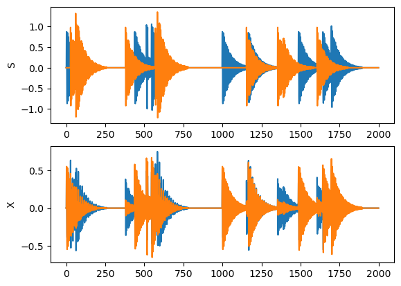
# Make mixed signals of two decaying tones
D = 2  # channels
N = 2000  # signal length
# Source signal
S = np.zeros((N, D))
for i in range(D):
    T = 200  # tone length
    M = 10  # number of tones
    t = np.arange(T)
    s = np.exp(-t/50)*np.sin(0.5*(2+i)*t)  # single tone
    ts = np.random.randint(0, N-T, M)  # start timing
    for m in range(M):
        S[ts[m]:ts[m]+T,i] += s  # add shifted tone
plt.subplot(2, 1, 1)
plt.plot(S)
plt.ylabel("S");
# Mixed signal
A = np.random.random((D,D))   # random matrix
print(A)
X = S@A.T
plt.subplot(2, 1, 2)
plt.plot(X)
plt.ylabel("X");
[[0.44689414 0.39050134]
 [0.62825702 0.10819952]]
# Applyy ICA to the mixture
W = np.eye(D)
for k in range(10):
    W = ica(X, W, alpha=0.001)
    print(W@A)
U = X@W.T
Y = np.tanh(U)
[[1.97998769 2.2567755 ]
 [3.23034136 0.22889848]]
[[ 1.1334797   7.01679679]
 [ 7.10263905 -0.98670735]]
[[ 0.01656438 10.23671404]
 [ 8.65947371 -0.12796697]]
[[-0.08206103 10.80105375]
 [ 8.87410954  0.01526071]]
[[-0.08657367 10.8671848 ]
 [ 8.89791222  0.02117864]]
[[-0.0867603  10.87452938]
 [ 8.90048213  0.02138424]]
[[-0.08676909 10.87534043]
 [ 8.90075852  0.02139023]]
[[-0.08676962 10.87542994]
 [ 8.90078822  0.02139027]]
[[-0.08676967 10.87543982]
 [ 8.90079141  0.02139025]]
[[-0.08676967 10.87544091]
 [ 8.90079175  0.02139025]]
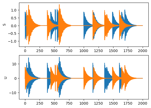
# plot the original and separated signals
plt.subplot(2, 1, 1)
plt.plot(S)
plt.ylabel("S")
plt.subplot(2, 1, 2)
plt.plot(U)
plt.ylabel("U");
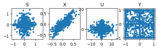
# plot t2D signal distributions
plt.subplot(1, 4, 1)
plt.plot(S[:,0], S[:,1], '.')
plt.axis('square')
plt.title("S")
plt.subplot(1, 4, 2)
plt.plot(X[:,0], X[:,1], '.')
plt.axis('square')
plt.title("X")
plt.subplot(1, 4, 3)
plt.plot(U[:,0], U[:,1], '.')
plt.axis('square')
plt.title("U")
plt.subplot(1, 4, 4)
plt.plot(Y[:,0], Y[:,1], '.')
plt.axis('square')
plt.title("Y");
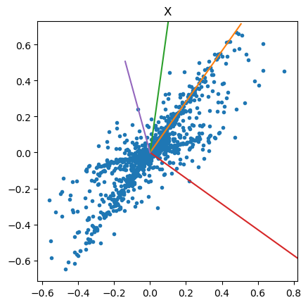
# see how the mixing and separation weights are aligned to mixed data
plt.plot(X[:,0], X[:,1], '.')
plt.axis('square')
plt.title("X")
# estimated mixing vectors
a = np.linalg.inv(W)
a = a/np.max(abs(a))
plt.plot([0, a[0,0]], [0, a[0,1]])
plt.plot([0, a[1,0]], [0, a[1,1]])
# separating vectors
w = W/np.max(W)
plt.plot([0,w[0,0]], [0,w[0,1]])
plt.plot([0,w[1,0]], [0,w[1,1]]);
Playing sound#
Do you want to hear the mixed and separated sounds?
You can use IPython.display library to play sound.
https://ipython.readthedocs.io/en/stable/api/generated/IPython.display.html
import IPython.display as ipd
# Source sounds
for i in range(D):
    ipd.display(ipd.Audio(S[:,i], rate=4000))  # 4kHz sampling
# Mixed sounds
for i in range(D):
    ipd.display(ipd.Audio(X[:,i], rate=4000))
# Separated sounds
for i in range(D):
    ipd.display(ipd.Audio(U[:,i], rate=4000))
Receptive fields of visual cortex neurons#
Cat visual cortex (Hubel & Wiesel)
Self-organization (von der Malsburgh)
by Informax (Linsker)
by SOM (Obermayer et al.)
by PCA (Sanger et al.)
by ICA (Bell & Sejnowski)
Replicating receptive field tuning#
Sanger (1989) applied generalized Hebbian learning to patches from natural images as inputs. The PCs learned as the input weights were similar to the receptive field propertis of visual cortical neurons.
References#
Bishop CM (2006) Pattern Recognition and Machine Learning. Springer. https://www.microsoft.com/en-us/research/people/cmbishop/prml-book/
Chapter 9: Mixture models and EM
Chapter 12: Continuous latent variables
Murphy K (2012) Machine learning: A probabilistic perspective. MIT press. https://probml.github.io/pml-book/
Chapter 25.2: Dirichlet process mixture models
Self Organization#
Hubel DH, Wiesel TN (1959). Receptive fields of single neurones in the cat’s striate cortex. Journal of Physiology, 148, 574-91. http://doi.org/10.1113/jphysiol.1959.sp006308
Hubel DH, Wiesel TN (1962). Receptive fields, binocular interaction and functional architecture in the cat’s visual cortex. Journal of Physiology, 160, 106-154. http://doi.org/10.1113/jphysiol.1962.sp006837
von der Malsburg C (1973). Self-organization of orientation sensitive cells in the striate cortex. Kybernetik, 14, 85-100. https://doi.org/10.1007/BF00288907
Kohonen T (1982). Self-Organized Formation of Topologically Correct Feature Maps. Biol Cybern, 43, 59-69. https://doi.org/10.1007/BF00337288
Olshausen BA, Field DJ (1996). Emergence of simple-cell receptive field properties by learning a sparse code for natural images. Nature, 381, 607-9. https://doi.org/10.1038/381607a0
Rao RP, Ballard DH (1999). Predictive coding in the visual cortex: a functional interpretation of some extra-classical receptive-field effects. Nat Neurosci, 2, 79-87. https://doi.org/10.1038/4580
PCA#
Sanger TD (1989). Optimal unsupervised learning in a single-layer linear feedforward neural network. Neural Networks, 2, 459-473. http://doi.org/10.1016/0893-6080(89)90044-0
Turk M, Pentland A (1991). Eigenfaces for recognition. Journal of Cognitive Neurosciece, 3, 71-86. http://doi.org/10.1162/jocn.1991.3.1.71
Infomax and ICA#
Linsker R (1986). From basic network principles to neural architecture. Proceedings of the National Academy of Sciences, USA, 83, 7508-7512, 8390-8394, 8779-8783. http://doi.org/10.1073/pnas.83.19.7508
Bell AJ, Sejnowski TJ (1995). An information-maxization approach to blind separation and blind deconvolution. Neural Comput, 7, 1129-1159. http://doi.org/10.1162/neco.1995.7.6.1129
Bell AJ, Sejnowski TJ (1997). The “independent components” of natural scenes are edge filters. Vision Research, 37, 3327-3338. http://doi.org/10.1016/s0042-6989(97)00121-1
Amari S (1998). Natural gradient works efficiently in learning. Neural Comput, 10, 251-276. http://doi.org/10.1162/089976698300017746