Appendix: Bayesian Model Fitting by PyStan#
Stan and PyStan#
Stan is a probabilistic programming language for probabilistic sampling and inference, including MCMC.
Stan uses an efficient MCMC algorithm Hamiltonian Monte Carlo (HMC) by default.
https://mc-stan.org
Stan is implemented by C++ and PyStan is a Python interface for Stan.
https://pystan.readthedocs.io
Installing PyStan#
PyStan is supported for Linux and macOS with C++ complier.
To use PyStan with Jupyter notebook, you need to install httpstan.
For Intel CPU machines, just pip install should work.
pip install httpstan
For Apple Silicone, you need to build from the source.
Download the souce code from GitHub
stan-dev/httpstan
and install as guided in
https://httpstan.readthedocs.io/en/latest/installation.html
Then you can install pystan and a visualization tool arviz by
pip install pystan arviz
Import libraries#
import numpy as np
import scipy.stats as stats
import matplotlib.pyplot as plt
%matplotlib inline
import stan
# For multichain MCMC
import multiprocessing
multiprocessing.set_start_method("fork")

import arviz
# For running PyStan via Jupyter Notebook
import nest_asyncio
nest_asyncio.apply()
Data sampling#
Here is a simple example of sampling data from a Gaussian distribution by PyStan.
# make a normal distribution model
model = stan.build('parameters {real x;} model {x ~ normal(0,1);}', random_seed=1)
Building: found in cache, done.
# see the organization of the model
model
Model(model_name='models/loo4gezv', program_code='parameters {real x;} model {x ~ normal(0,1);}', data={}, param_names=('x',), constrained_param_names=('x',), dims=([],), random_seed=1)
# take 1000 samples
sample = model.sample(num_chains=1, num_samples=1000, num_warmup=100)
print(sample)
print(sample['x'].shape)
Sampling: 0%
Sampling: 100%, done.
Messages received during sampling:
Gradient evaluation took 5e-06 seconds
1000 transitions using 10 leapfrog steps per transition would take 0.05 seconds.
Adjust your expectations accordingly!
WARNING: There aren't enough warmup iterations to fit the
three stages of adaptation as currently configured.
Reducing each adaptation stage to 15%/75%/10% of
the given number of warmup iterations:
init_buffer = 15
adapt_window = 75
term_buffer = 10
<stan.Fit>
Parameters:
    x: ()
Draws: 1000
(1, 1000)
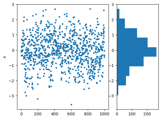
# see the samples
plt.subplot(1,3,(1,2))
plt.plot(sample['x'][0], '.');
plt.ylabel('x')
# show the histogram
plt.subplot(1,3,3)
plt.hist(sample['x'][0], orientation='horizontal');
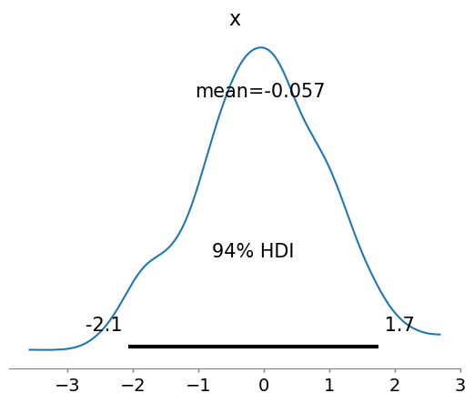
# plot the sample distribution
arviz.plot_posterior(sample, var_names=['x']);
General steps for Bayesian modeling with stan#
Describing a probabilistic generative model using Stan language.
Compiling a Stan file.
Running MCMC to obtain posterior samples.
Diagnosing the validity of MCMC.
Evaluating an obtained posterior.
Example 1: Coin-toss#
Let us first see a very basic example of coin toss.
Head (\(x=1\)) and tail (\(x=0\)) follows a Bernoulli distribution: $\( x \sim \mbox{Bernoulli}(\mu) \)\( where \)\mu\( is the mean parameter \)0 \le \mu \le 1$.
A common prior distribution for \(\mu\) is the Beta distribution \(\mbox{Beta}(x, a, b) \sim x^{a-1} (1-x)^{b-1}\).
For \(n\) coin tosses, the number of heads \(x\) follows a binomial distribution: $\( x \sim \mbox{Binomial}(n, \mu) \)$
Step 1: Describing a probabilistic generative model using Stan language#
Here we are interested to estimate the mean parameter \(\mu\) from samples.
stan_coin_toss = """
data {
    int<lower=0> n; // Number of tosses
    int<lower=0> x; // Number of heads
    int<lower=0> a; // Parameter "a" of the prior (Beta Distribution)
    int<lower=0> b; // Parameter "b" of the prior (Beta Distribution)
}

parameters {
    real<lower=0, upper=1> mu;
}

model {
    mu ~ beta(a, b); // Write a prior distribution
    x ~ binomial(n, mu);
}
"""
n = 100    # Number of tosses
x = 60     # Number of heads
a = 2     # Parameter "a" of the prior (Beta Distribution)
b = 4     # Parameter "b" of the prior (Beta Distribution)
data_coin_toss = {
    "n": n,
    "x": x,
    "a": a,
    "b": b
}
Step 2: Compiling a Stan file#
posterior = stan.build(stan_coin_toss, data=data_coin_toss, random_seed=1)
Building: found in cache, done.
Messages from stanc:
Warning: The parameter mu has 2 priors.
Step 3: Running MCMC to obtain posterior samples#
# take samples
fit = posterior.sample(num_chains=4, num_samples=2000, num_warmup=100)
fit
Sampling: 0%
Sampling: 25% (2100/8400)
Sampling: 50% (4200/8400)
Sampling: 75% (6300/8400)
Sampling: 100% (8400/8400)
Sampling: 100% (8400/8400), done.
Messages received during sampling:
Gradient evaluation took 5e-06 seconds
1000 transitions using 10 leapfrog steps per transition would take 0.05 seconds.
Adjust your expectations accordingly!
WARNING: There aren't enough warmup iterations to fit the
three stages of adaptation as currently configured.
Reducing each adaptation stage to 15%/75%/10% of
the given number of warmup iterations:
init_buffer = 15
adapt_window = 75
term_buffer = 10
Gradient evaluation took 4e-06 seconds
1000 transitions using 10 leapfrog steps per transition would take 0.04 seconds.
Adjust your expectations accordingly!
WARNING: There aren't enough warmup iterations to fit the
three stages of adaptation as currently configured.
Reducing each adaptation stage to 15%/75%/10% of
the given number of warmup iterations:
init_buffer = 15
adapt_window = 75
term_buffer = 10
<stan.Fit>
Parameters:
    mu: ()
Draws: 8000
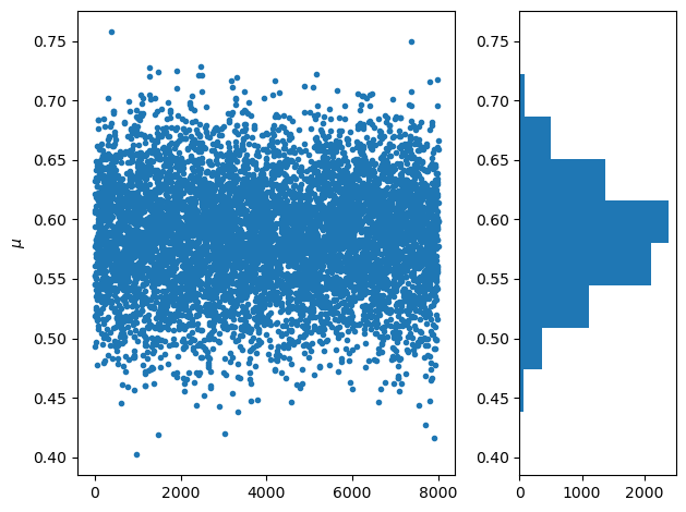
# see the sampled parameters
plt.subplot(1,3,(1,2))
plt.plot(fit['mu'][0], '.')
plt.ylabel(r'$\mu$')
# show the histogram
plt.subplot(1,3,3)
plt.hist(fit['mu'][0], orientation='horizontal')
plt.tight_layout()
Step 4: Diagnosing the validity of MCMC#
The essential point is whether a simulated chain is converged to a stationary process. A simple method to diagnose the convergence is to calculate the Gelman-Rubin statistic (a.k.a. Rhat).
You can easily calculate it (and another statistic called effective sample size (ESS)) by using Arviz.
Rhat of converged samples becomes 1. The Stan development team says that the diagnosis is accepted if Rhat is between 1 and 1.05 but there is open to debate.
ESS is for evaluating whether there is autocorrelation within a chain. If ESS is larger than sample size of each chain, it is proved that autocorrelation is small enough.
arviz.summary(arviz.from_pystan(posterior=fit, posterior_model=posterior))
| mean | sd | hdi_3% | hdi_97% | mcse_mean | mcse_sd | ess_bulk | ess_tail | r_hat | |
|---|---|---|---|---|---|---|---|---|---|
| mu | 0.584 | 0.046 | 0.496 | 0.67 | 0.001 | 0.0 | 3115.0 | 4972.0 | 1.0 |
It is also good to check a convergence by your eyes. If you simulate multiple chains, it is important to check whether there is not big shape difference among posterior distributions from the chains.
arviz.plot_trace(fit, var_names=('mu'), combined=False);
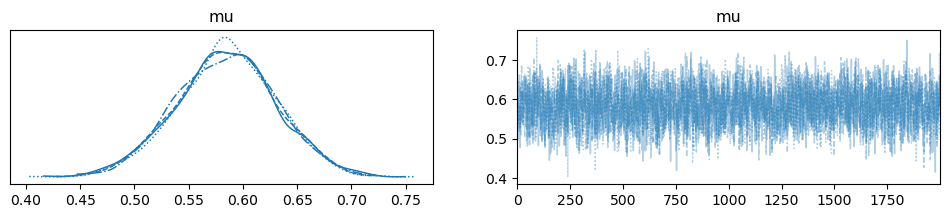
If MCMC is not converged, the following solutions (and more) are considered.
Increasing burn-in samples
Increasing the number of chains
Reconsidering a model structure
Step 5: Evaluating an obtained posterior#
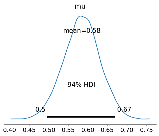
Highest density interval (HDI): All points within HDI have a higher probability density than points outside the interval. The HDI can be used in the context of uncertainty characterisation of posterior distributions as Credible Interval (CI).
arviz.plot_posterior(fit, var_names=['mu']);
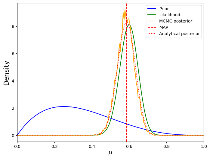
This example is simple enough to compute a posterior analytically. Let’s see how close the MCMC posterior is to the analytical posterior.
mus = np.linspace(0, 1, 200)
prior = stats.beta(a, b)
post = stats.beta(a+x, b+n-x)
post_hist = np.histogram(fit['mu'], bins=mus)
post_dist = stats.rv_histogram(post_hist)

plt.figure(figsize=(8, 6))
plt.plot(mus, prior.pdf(mus), label='Prior', c='blue')
plt.plot(mus, n*stats.binom(n, mus).pmf(x), label='Likelihood', c='green')
plt.plot(mus, post_dist.pdf(mus), label='MCMC posterior', c='orange')
plt.axvline((x+a-1)/(n+a+b-2), label='MAP', c='red', ls='dashed')
plt.plot(mus, post.pdf(mus), label='Analytical posterior', c='red', ls='dotted')
# plt.axvline(mu/n, c='green', linestyle='dashed', alpha=0.4, label='MLE')
plt.xlim([0, 1])
plt.xlabel(r'$\mu$', fontsize=14)
plt.ylabel('Density', fontsize=16)
plt.legend()
plt.show()
References#
Carpenter B, Gelman A, Hoffman MD, Lee D, Goodrich B, Betancourt M, Brubaker M, Guo J, Li P, Riddell A (2017). Stan: A Probabilistic Programming Language. Journal of Statistical Software, 76. https://doi.org/10.18637/jss.v076.i01
Stan web site: https://mc-stan.org
PyStan readthedocs: https://pystan.readthedocs.io/en/latest/