Introduction
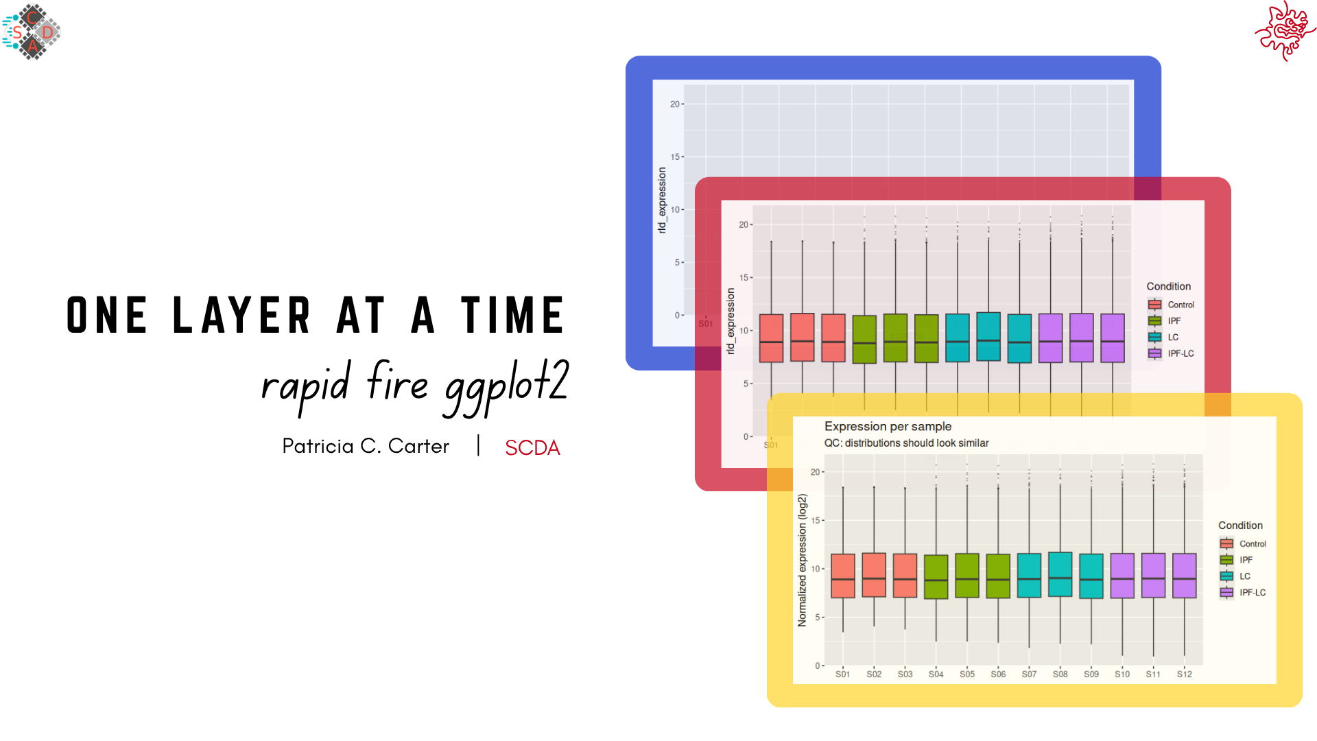
This tutorial is a short introduction to data visualization using R’s ggplot2 package. It is aimed at those with some working knowledge of R and serves as a natural follow-up to the Introduction to R Programming workshop. The tutorial is a quick survey of creating plots one layer at a time.
Here is how it works:
- R runs inside your web browser, so you don’t need to install anything. The first time you click Run Code, R takes a few seconds to load.
- To run an exercise, click Run Code. Code chunks can be edited and re-run. Start Over brings back the original code.
- New lines within the code chunks are marked with
#NEW LINE. - Some code chunks contain a blank to fill in,
______. If you get stuck, use Show Hint, then Show Solution.
The main layers of your plot
Every ggplot requires 3 components (Wickham, Navarro & Pedersen, ggplot2: Elegant Graphics for Data Analysis, 3e, §2.3):
- Data: the data frame.
- Aesthetic mappings, written as
aes(): these are the columns in the data frame you want to visualize (e.g.x,y,fill,colour). - At least one layer:
geom_*(), which decides which plot type is used to draw the data (e.g.geom_point(),geom_bar(),geom_boxplot()).
Exploring the data
Before we start, let’s explore the first 10 rows of our expr data object.
Our expr object contains simulated data from an RNA-seq experiment measuring gene expression under two conditions, knockout and wildtype
Again, these data are simulated and are not biologically realistic
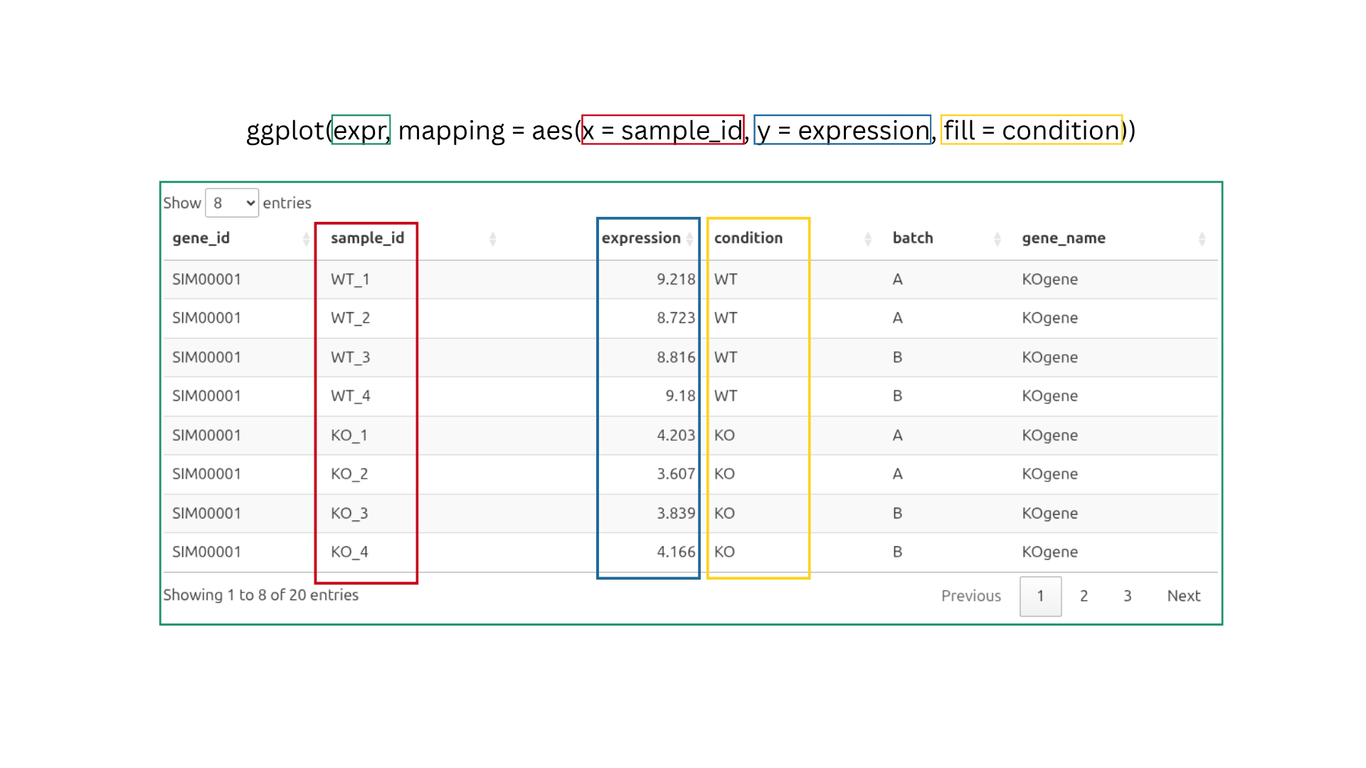
To demonstrate, we will first run a plot with only two components, data and aesthetic mappings. Our data is the expr data frame, and the aesthetic mappings use the sample ID column as x and the expression values as y.
We also want to separate our conditions with fill = condition, which gives WT and KO different colors.
Question: Why is the data not showing up on the plot?
- The data did not load.
fillcannot be used withsample_id.- ggplot knows the axes, but no layer tells it how to draw the data.
- A theme is needed before anything is shown.
TipCheck your answer
ggplot knows the axes, but no layer tells it how to draw the data.
Explanation
The ggplot() function stores the data. It tells ggplot which data to use and which columns go where. In the code above, ggplot(expr, mapping = aes(x = sample_id, y = expression, fill = condition)), we told ggplot to use the expr data frame, put sample_id on the x-axis, put expression on the y-axis, and color by condition.
That’s enough for ggplot to draw the axes, but we haven’t told it what shape to use for the data(bars, points, lines, etc.).
Adding a layer
For the plot to be drawn, we need the third component, a layer. A layer such as geom_*() determines how the data will be drawn (e.g. as a box, a point, a bar or a line).
Let’s add geom_boxplot() as a new layer to draw the distribution of expression values for each sample.
In ggplot2, we use the plus sign + to add a new layer to the plot.
The plus sign + always goes at the end of the previous line, never at the beginning of the next.
Changing aesthetics
Anything written inside aes() is a mapping: the appearance depends on a column (fill = condition gives WT and KO different colors). Anything written outside aes(), directly in geom_*(), is a setting and is a fixed value for everything. For example, outlier.colour = "grey20" makes every outlier dark grey.
Outliers are drawn by the boxplot, so their size, transparency (alpha, from 0 = invisible to 1 = solid) and color are settings of geom_boxplot().
Choosing your own colors
fill = condition tells ggplot which boxes get different colors, but ggplot2 chooses the colors. To pick them yourself, add a scale such as scale_fill_*(). scale_fill_manual() lets you supply a vector of colors of your choosing.
To save you some typing, this tutorial has already created a color vector called condition_colors behind the scenes. You won’t see the code that made it, but it looks like this:
condition_colors <- c("WT" = "#1a80bb", "KO" = "#a00000")A quick note on colors:
"#1a80bb" and "#a00000" are hex codes for the colors we selected, in this case blue and red. See the R Graph Gallery for more examples and resources on selecting colors in ggplot2.
Fill in the blank to use it.
The scale needs the named vector of colors from the setup. Its name starts with condition_.
ggplot(expr, mapping = aes(x = sample_id, y = expression, fill = condition)) +
  geom_boxplot(outlier.size = 0.2, outlier.alpha = 0.3, outlier.colour = "grey20") +
  scale_fill_manual(values = condition_colors)
Labels
labs() sets the plot title, the axis titles and the legend titles. The name of each argument matches the aesthetic it labels, so fill = labels the fill legend.
x = NULL removes the x-axis title completely. In this example, the sample names already say enough.
Give the plot the title “KO vs WT Expression” and the legend the title “Condition”.
Both blanks are text, so they need quotation marks, "like this".
ggplot(expr, mapping = aes(x = sample_id, y = expression, fill = condition)) +
  geom_boxplot(outlier.size = 0.2, outlier.alpha = 0.3, outlier.colour = "grey20") +
  scale_fill_manual(values = condition_colors) +
  labs(
    title = "KO vs WT Expression",
    x = NULL,
    y = "Expression",
    fill = "Condition"
  )
Themes
A theme controls everything that is not data: background, gridlines, fonts, legend position, axis text. Complete themes such as theme_minimal(), theme_light() and theme_classic() change all of these at once. To change only specific parts of the plot, use theme(), shown in the next step.
Try: replace theme_minimal() with theme_classic() or theme_bw().
Changing text appearance in theme()
To change single elements, use theme().
Text elements are changed with element_text() inside the theme() function:
hjustis horizontal justification: 0 = left, 0.5 = center, 1 = right.anglerotates the text. At 45°,hjust = 1lines up the end of each label with its tick mark.
Try: change the horizontal justification hjust = of the x-axis text to see how the labels move relative to the tick marks.
Order is important
In ggplot2, the order in which you add theme elements matters, because a complete theme added later overrides earlier styling.
For example, we previously rotated the x-axis text to 45° and centered the plot title. If we placed these adjustments before a complete theme such as theme_minimal(), they would be overridden by the styles that theme_minimal() brings in.
To keep your customizations, add the complete theme first and your theme() adjustments after it.
The code below draws the same plot twice. On the left, theme() comes after theme_minimal(), and on the right, it comes before.
Run it and compare.
Fill vs. colour
Boxes have two color aesthetics:
fill: the inside of the box.colour: the outline, the whiskers and the median line.
First, make the fill semi-transparent with alpha = 0.4. This is a setting, so it goes inside geom_boxplot() and outside aes().
Now we will map the outline color to condition as well and give it the same colors.
Ready-made palettes
Instead of choosing colors by hand, you can use a ready-made palette. The scale_*_brewer() scales use the ColorBrewer palettes. For example, "Set1" is designed for categories such as WT and KO.
Only the two scale lines change.
Try: palette = "Set2" or palette = "Dark2".
Your turn
Previously, we made one box per sample. Make a boxplot from scratch that shows one box per condition, so that all wild-type (WT) values go in one box and all knockout (KO) values go in the other.
Your plot should have:
conditionon the x-axis andexpressionon the y-axis- boxes filled by condition (use
fill, notcolour, becausecolouronly changes the outline) - the title “Expression by Condition”, centered
- no x-axis title
theme_classic()
If you like, also bring over the styling from earlier steps (outlier appearance, condition_colors, axis and legend labels).
Start from your code in the “Changing text appearance” step. Change x = sample_id to x = condition. You can delete the angled axis-label code.
x = NULL inside labs() removes the axis title completely. Titles are left-aligned by default. Center the title with this, and put it after theme_classic(), otherwise theme_classic() overwrites it.
theme(plot.title = element_text(hjust = 0.5))ggplot(expr, mapping = aes(x = condition, y = expression, fill = condition)) +
geom_boxplot(outlier.size = 0.2, outlier.alpha = 0.3, outlier.colour = "grey20") +
scale_fill_manual(values = condition_colors) +
labs(
title = "Expression by Condition",
x = NULL,
y = "Expression",
fill = "Condition"
) +
theme_classic() +
theme(
plot.title = element_text(hjust = 0.5)
)Volcano plot
Points
A volcano plot shows every gene as one point:
- x-axis:
log2FoldChange, the change in expression. - y-axis:
-log10(padj), how significant the change is. You can use any mathematical expression in your plot code.-log10()turns small p-values into large numbers, so the most significant genes sit at the top.
The geom is geom_point(). It draws each row as a separate point, and depending on your data, some points may overlap.
Colors
For geom_point(), points are colored with colour, not fill, so the scale is scale_colour_manual().
Let’s start by pairing each category with a color, where:
- Down = downregulated genes
- Up = upregulated genes
- NS = not significant genes
volcano_colors <- c("Down" = "#4647AE", "NS" = "grey80", "Up" = "darkred")Fill in the blank to use it.
The scale needs the named vector of colors from the setup. Its name starts with volcano_.
ggplot(volcano, mapping = aes(x = log2FoldChange, y = -log10(padj), colour = diffexpr)) +
  geom_point(alpha = 0.4) +
  scale_colour_manual(values = volcano_colors)
Cut-off lines
Genes are called significant when they pass two cut-offs. For this tutorial, we have already created the p-value and fold-change cut-offs as two objects:
geom_hline()draws a horizontal line at the p-value cut-off. We use-log10(p_cut)because the y-axis is on that scale.geom_vline()draws vertical lines at the fold-change cut-offs, one on each side of zero.
Side note: the base R function c(...) combines values into a single vector. For example, if fc_cut is 1, then c(-fc_cut, fc_cut) gives c(-1, 1). geom_vline() draws one line for each value in xintercept, which gives us two lines.
Try: linetype = "solid" or "dotted".
Theme
theme_light() gives a white background with light grey gridlines.
Labels with math
Sometimes we want to improve readability by adding subscripts to our labels. For this we use the expression() function (not related to the expression column in the expr data).
Inside expression():
[ ]makes a subscript, solog[2]is log₂.~adds a space.*joins two pieces with no space.
To learn more about mathematical annotation, see the plotmath documentation.
colour = NULL removes the legend title.
As before, the title is centered with theme(), after the complete theme.
Labelling genes of interest
To label only a few genes, add a layer that uses its own data. The data = argument of a geom replaces the plot’s data for that layer only. Here we give it only the rows for our genes of interest.
aes(label = gene_name) inside the layer is a local mapping, so it applies only to this layer. The mappings in ggplot() are global and apply to every layer.
geom_label_repel() (from the ggrepel package) moves labels so they don’t overlap. show.legend = FALSE stops it from adding a letter “a” on top of the legend keys. #Again need to explain this better…
Side note: data = volcano[volcano$gene_name %in% genes_interest, ] tells this layer to use only our genes of interest, instead of the whole data set as before.
Your turn
Fill in the blanks to finish the volcano plot. Your plot should:
- label the 10 most significant genes (the 10 smallest
padjvalues) - use
theme_classic(), with the title still centered - show the legend at the bottom
- have bigger axis titles (pick your own size)
One new tool: order() gives the row positions from smallest to largest value. Combined with [ ], it sorts a data frame, and [1:10] keeps the first 10:
data[order(data$column)[1:10], ]- Blank 1:
order()needs a column, written asdata$column. - Blank 2: the label layer uses its own small data frame. Which one did you just make?
- Blank 3: the complete theme goes here, before
theme(). - Blank 4: any number, try 14.
- Blank 5: the position is text, so it needs quotation marks.
top_genes <- volcano[order(volcano$padj)[1:10], ]

ggplot(volcano, mapping = aes(x = log2FoldChange, y = -log10(padj), colour = diffexpr)) +
  geom_point(alpha = 0.6) +
  geom_hline(yintercept = -log10(p_cut), linetype = "dashed", colour = "#141414", linewidth = 0.5) +
  geom_vline(xintercept = c(-fc_cut, fc_cut), linetype = "dashed", colour = "#141414", linewidth = 0.5) +
  geom_label_repel(
    data = top_genes,
    aes(label = gene_name),
    show.legend = FALSE,
    size = 5,
    min.segment.length = 0,
    max.overlaps = Inf     # draw all 10 labels, even if crowded
  ) +
  scale_colour_manual(values = volcano_colors) +
  guides(colour = guide_legend(override.aes = list(alpha = 1, size = 4))) +  # solid, larger legend dots
  labs(
    title = "My Volcano Plot",
    x = expression(log[2]~"FC"),
    y = expression("-Log"[10]*"(padj)"),
    colour = NULL
  ) +
  theme_classic() +
  theme(
    plot.title = element_text(hjust = 0.5, size = 19),
    axis.title = element_text(size = 14),   # both axis titles
    legend.position = "bottom"
  )
Bar charts
Which geom_*() you use for a bar chart depends on whether your data already contains the bar heights. See the ggplot2 documentation for a more detailed explanation.
geom_bar()counts the rows in each group and uses that count as the bar height. By default it usesstat_count().geom_col()uses a value already in the data as the bar height.
Our read_summary data already contains the number of reads (reads_M, millions of reads), so we use geom_col(). With fill = category, each bar is split into categories. The position argument decides how:
position = "stack"keeps the real totals. This is the default.position = "fill"stretches every bar to 100%.position = "dodge"places the bars side by side.
From here on, we leave out mapping =. aes() is the second argument of ggplot(), so R matches it without the name.
Run the stacked version first.
Now change the position so every bar shows proportions.
Use the option that stretches every bar to 100%. The position is text, so it needs quotation marks.
ggplot(read_summary, aes(x = sample_id, y = reads_M, fill = category)) +
  geom_col(position = "fill")
Percentages on the axis
With position = "fill", the y-axis runs from 0 to 1. scales::percent changes these labels to percentages.
The scales:: prefix means “use the percent function from the scales package” without loading the whole package with library(). The scales package is installed together with ggplot2.
Your turn
We created a color vector called read_colors, with one color per category.
read_colors <- c("Assigned" = "#0072B2", "Multimapped" = "#A8DF8E", "Unassigned" = "lightgrey")Your plot should:
- use
read_colorsfor the category colors - have a centered title
- have no x-axis title
- have a more readable y-axis title, such as “Percentage of Reads”
- use a complete theme of your choice
- The scale needs the named vector of colors from the setup. Its name starts with
read_. - Use the
labs()function to add the title and axis titles.NULLremoves a title. - Add a complete theme, such as
theme_classic(). - Center the title with
element_text()insidetheme().
ggplot(read_summary, aes(x = sample_id, y = reads_M, fill = category)) +
  geom_col(position = "fill") +
  scale_y_continuous(labels = scales::percent) +
  scale_fill_manual(values = read_colors) +
  labs(
    title = "Bar Plot",
    y = "Percentage of Reads",
    x = NULL
  ) +
  theme_classic() +
  theme(plot.title = element_text(hjust = 0.5))
Line graph
Lines
The weights_mean object has already been summarized. It contains one row per condition per week, with the mean weight (mean_weight) and its standard error (se).
geom_line() connects the points in order along the x-axis. Because colour = condition is mapped, ggplot draws one line per condition.
Points and error bars
To draw points and error bars, we add two more layers to the same plot, geom_point() and geom_errorbar().
In geom_point(), size = 2 is a setting, so every point gets the same size.
geom_errorbar() needs two extra aesthetics, ymin and ymax, the bottom and top of each bar. We map them inside geom_errorbar(), so they apply only to that layer. The x, y and colour mappings in ggplot() are global and shared by all three layers.
width = 0.2 is a setting for the width of the whisker caps.
Labels and theme
We will now add the title “Mean Weights”, center it and name the axes. colour = NULL removes the legend title.
Try: add colour = "darkgreen" inside geom_line(). What happens to the two lines, and why? (Hint: setting vs. mapping.)
Session info
Click Run Code to list the R version and packages running in your browser. If you run the same code on your own computer, your versions may be different, which can change how some plots look.
About this tutorial
Written by Patricia C. Carter, Scientific Computing & Data Analysis (SCDA), OIST.
Last updated October 2026.
Source code: https://github.com/oist/ggplot2_workshop_interactive